JavaScript / ES6+ Bootcamp – Lesson 1

The goal of this lesson is simple: understand what JavaScript is actually doing when you write basic code.

Coming from Ruby, you’ll notice that many concepts are similar, but JavaScript has some syntax and behavior that becomes important later in React and Node.js.

Variables, Values, Objects, Arrays, Functions and Return Values

1. Variables: let and const

In modern JavaScript, primarily use:

const name = "Abhilash";
let age = 40;

Think of them roughly like Ruby local variables:

name = "Abhilash"
age = 40

The difference is important:

const

The variable cannot be reassigned:

const name = "Abhilash";
name = "John"; // TypeError

let

The variable can be reassigned:

let age = 40;
age = 41;

What about var?

You’ll see:

var name = "Abhilash";

in older JavaScript code.

For modern JavaScript:

Use const by default.
Use let when reassignment is required.
Avoid var unless you're dealing with legacy code.

2. Everything starts with values

JavaScript variables hold values.

const name = "Abhilash";
const age = 40;
const active = true;

These values have types.

typeof name; // "string"
typeof age; // "number"
typeof active; // "boolean"

Some common types:

string
number
boolean
undefined
null
object
symbol
bigint

For now, focus on:

string
number
boolean
undefined
null
object

3. Arrays

An array stores multiple values.

const numbers = [10, 20, 30];

You can access them using an index:

numbers[0]; // 10
numbers[1]; // 20
numbers[2]; // 30

Just like Ruby:

numbers = [10, 20, 30]
numbers[0] # 10

JavaScript arrays are zero-indexed too.

Important

This:

const numbers = [10, 20, 30];

means numbers contains one array value.

It does not mean:

numbers = 10
20
30

Think:

numbers
|
v
[10, 20, 30]

4. Objects

JavaScript objects are heavily used in React and Node.

const user = {
id: 1,
name: "Abhilash",
active: true
};

You can access properties:

user.name; // "Abhilash"
user.id; // 1
user.active; // true

Ruby equivalent:

user = {
id: 1,
name: "Abhilash",
active: true
}
user[:name]

JavaScript also supports bracket notation:

user["name"];

This becomes useful when the property name is dynamic.


5. Arrays can contain objects

This is extremely common in React.

const users = [
{ id: 1, name: "John" },
{ id: 2, name: "Jane" },
{ id: 3, name: "Mike" }
];

Visualize it:

users
|
v
[
{ id: 1, name: "John" },
{ id: 2, name: "Jane" },
{ id: 3, name: "Mike" }
]

Then:

users[0].name;

returns:

"John"

This structure is everywhere in frontend applications.


6. Functions

A JavaScript function can be written like:

function add(a, b) {
return a + b;
}

Call it:

const result = add(10, 20);
console.log(result); // 30

Ruby equivalent:

def add(a, b)
a + b
end
result = add(10, 20)

So far, very familiar.


7. The important idea: functions are values

This is one of the biggest concepts you need for React and Node.

In JavaScript:

function add(a, b) {
return a + b;
}

The function itself is a value.

You can store it:

const operation = add;

Now:

operation(10, 20);

returns:

30

Visualize:

add
|
v
function
operation
|
+------> same function

This is why JavaScript can pass functions around so easily.


8. Functions can return anything

A function can return a number:

function getAge() {
return 40;
}

A string:

function getName() {
return "Abhilash";
}

An object:

function getUser() {
return {
id: 1,
name: "John"
};
}

An array:

function getUsers() {
return [
{ id: 1, name: "John" },
{ id: 2, name: "Jane" }
];
}

And importantly, a function can return another function:

function createGreeter() {
return function() {
console.log("Hello");
};
}

We’ll use this concept later when learning closures.


9. This explains useState

Now let’s return to the example that confused you:

const [users, setUsers] = useState([]);

Ignore React for a moment.

Imagine an ordinary function:

function useState(initialValue) {
return [
initialValue,
function setValue(value) {
console.log(value);
}
];
}

Now call:

const result = useState([]);

What does result contain?

Conceptually:

[
[],
setValueFunction
]

So:

const users = result[0];
const setUsers = result[1];

Now combine the two operations with destructuring:

const [users, setUsers] = result;

Therefore:

const [users, setUsers] = useState([]);

means:

1. Pass [] into useState
2. useState returns [value, function]
3. destructure that returned array
4. users gets element 0
5. setUsers gets element 1

This is a critical mental model.


10. Array destructuring

Let’s isolate the JavaScript feature.

const numbers = [10, 20];
const [a, b] = numbers;

Equivalent to:

const a = numbers[0];
const b = numbers[1];

You can even ignore values:

const [first, , third] = [10, 20, 30];
console.log(first); // 10
console.log(third); // 30

11. Object destructuring

There is another extremely common form:

const user = {
name: "John",
age: 30
};
const { name, age } = user;

Equivalent to:

const name = user.name;
const age = user.age;

So remember:

Array -> []
Object -> {}

Therefore:

const [a, b] = array;
const { name, age } = object;

This distinction is extremely important in React.


12. Arrow functions

Modern JavaScript frequently uses:

const add = (a, b) => {
return a + b;
};

Short form:

const add = (a, b) => a + b;

Equivalent roughly to:

function add(a, b) {
return a + b;
}

React code uses arrow functions constantly:

users.map(user => user.name);

Don’t worry about map yet. Just notice:

user => user.name

is a function.


13. Why callbacks matter

Consider:

function execute(callback) {
callback();
}

Then:

execute(() => {
console.log("Hello");
});

What’s happening?

execute()
|
| receives a function
v
callback
|
v
callback()
|
v
console.log("Hello")

The function is being passed as a value.

This is the foundation of callbacks.

We’ll go much deeper into this in a later lesson.


Ruby developer mental model

For now, keep these mappings in your head:

JavaScriptRuby
const x = 10x = 10
[]Array
{}Hash-like object
functiondef / Proc/Lambda concepts
returnreturn
obj.nameobj[:name] for Hash
array[0]array[0]
function as valueProc/lambda/block-like concept
arrow functionlambda-ish syntax, but not identical

The last row is deliberately approximate. JavaScript functions, arrow functions, Ruby blocks, Procs and lambdas are not interchangeable concepts. We’ll cover the differences properly.


🎯 Lesson 1 int. questions

Try answering these without looking back.

Question 1

What does this return?

const numbers = [10, 20, 30];
numbers[1];

Question 2

What is the difference between:

const user = {
name: "John"
};

and:

const users = [
{ name: "John" }
];

Question 3

What does this do?

const [a, b] = [10, 20];

Question 4

What does this return?

function getUser() {
return {
id: 1,
name: "John"
};
}

Question 5

What is stored in operation?

function add(a, b) {
return a + b;
}
const operation = add;

Small exercise

Without running it, predict the output:

function getUser() {
return [
{ id: 1, name: "John" },
{ id: 2, name: "Jane" }
];
}
const users = getUser();
const [firstUser, secondUser] = users;
console.log(firstUser.name);
console.log(secondUser.name);

Then try this variation:

const [firstUser] = getUser();
console.log(firstUser.name);

The key skill I’m looking for is not memorizing syntax. It’s being able to mentally trace:

function call
↓
return value
↓
array/object
↓
destructuring
↓
variables

Once that becomes natural, a lot of React code will stop looking mysterious.

Next lesson: let, const, scope, hoisting, and why JavaScript behaves differently from Ruby around variable scope.

Happy Learning! to be continued..

Senior-Level Linux Commands Every Backend Engineer Should Know

For a senior backend engineer, Linux commands are more than tools for navigating directories.

They become a production debugging language.

When a Rails application is consuming too much memory, a log contains millions of lines, a deployment introduces unexpected configuration changes, or a background worker suddenly starts failing, knowing how to combine commands such as sed, awk, grep, find, xargs, sort, uniq, cut, tr, jq, and ps can save hours.

The real skill is not memorizing commands. It is understanding how to compose them into pipelines.

command1 | command2 | command3

This article focuses on commands and techniques that become particularly valuable at a senior engineering level.


1. grep – Search With Intent

Most developers know:

grep "ERROR" production.log

But grep becomes much more powerful with regular expressions and recursive searches.

Search recursively

grep -R "ActiveRecord::Deadlocked" log/

Useful when you don’t know which file contains the problem.

Ignore case

grep -Ri "timeout" .

Show line numbers

grep -n "connection refused" production.log

Search multiple patterns

grep -E "ERROR|FATAL|Exception" production.log

Show context around matches

grep -C 5 "NoMethodError" production.log

This is extremely useful for application logs because the surrounding lines often contain request IDs, parameters, stack traces, or timestamps.

When to use

Use grep when your primary operation is:

“Find lines matching this condition.”

2. sed – Stream Editing

sed is one of the most useful Linux commands for manipulating text without opening an editor.

The simplest example:

sed 's/foo/bar/g' file.txt

Replace every foo with bar.

Delete lines

Delete empty lines:

sed '/^$/d' file.txt

Delete lines containing DEBUG:

sed '/DEBUG/d' production.log

Print specific lines

sed -n '100,150p' production.log

This displays lines 100 through 150.

Very useful when investigating a specific portion of a huge log file.

Modify a configuration file

For example:

sed -i 's/RAILS_LOG_LEVEL=info/RAILS_LOG_LEVEL=debug/' .env

-i modifies the file in place.

Be careful with production configuration files. Prefer making a backup when appropriate:

sed -i.bak 's/old_value/new_value/g' config.yml

Advanced use: remove sensitive information

Suppose logs contain email addresses:

User login: john@example.com
User login: alice@example.com

We can mask them:

sed -E 's/[[:alnum:]._%+-]+@[[:alnum:].-]+\.[A-Za-z]{2,}/[REDACTED]/g' app.log

This is useful when sanitizing logs before sharing them.

When to use sed

Think:

“I want to transform or filter text while streaming it.”

3. awk – Lightweight Data Processing

awk is one of the most important commands for senior engineers.

It treats input as structured columns.

Suppose:

101 John 4500
102 Alice 6000
103 Bob 5000

Run:

awk '{print $1, $3}' users.txt

Output:

101 4500
102 6000
103 5000

Filter records

awk '$3 > 5000 {print $1, $2, $3}' users.txt

Now only users earning more than 5000 are printed.

Calculate values

awk '{sum += $3} END {print sum}' users.txt

Calculate the total salary.

Average:

awk '{sum += $3; count++} END {print sum/count}' users.txt

Processing logs

Imagine an Nginx log:

10.0.0.1 GET /users 200
10.0.0.2 GET /users 500
10.0.0.3 GET /products 200
10.0.0.4 GET /users 500

Extract HTTP status:

awk '{print $4}' access.log

Count status codes:

awk '{print $4}' access.log | sort | uniq -c

Result:

2 200
2 500

awk with conditions

awk '$4 >= 500 {print}' access.log

Find server errors.

When to use awk

Think:

“My input has columns/records and I need to filter, transform, aggregate, or calculate something.”

For quick operational data analysis, awk can often replace writing a small script.

4. cut – Extract Columns

For simple column extraction, cut is usually easier than awk.

Example:

cut -d',' -f1 users.csv

Extract the first CSV field.

Multiple fields:

cut -d',' -f1,3 users.csv

Character ranges:

cut -c1-10 file.txt

Use cut when the operation is straightforward.

Use awk when logic becomes conditional or computational.

5. sort + uniq – Finding Patterns

These commands become extremely powerful together.

Suppose you want to find the most common URLs:

awk '{print $7}' access.log |
sort |
uniq -c |
sort -nr

Example:

1500 /api/users
980 /api/orders
450 /health

This is a classic production-analysis pipeline.

Why sort before uniq?

uniq only detects adjacent duplicate lines.

Therefore:

sort file.txt | uniq

is usually required.

6. head and tail – Inspect Large Files Safely

Instead of opening a 10 GB log:

head -n 50 production.log

Last 100 lines:

tail -n 100 production.log

The real power is:

tail -f production.log

Follow new log entries in real time.

For Rails applications this is particularly useful during deployments:

tail -f log/production.log

You can combine it with grep:

tail -f production.log | grep --line-buffered "ERROR"

Now you’re effectively monitoring errors as they occur.

7. find – Locate Files Precisely

Find Ruby files:

find app/ -type f -name "*.rb"

Find files modified recently:

find log/ -type f -mtime -1

Find large files:

find /var/log -type f -size +500M

Find and execute a command:

find tmp/ -type f -name "*.tmp" -delete

Be careful with destructive commands.

A safer approach is:

find tmp/ -type f -name "*.tmp" -print

Inspect the result first.

8. xargs – Turn Output Into Arguments

Suppose:

find tmp/ -type f -name "*.tmp"

returns many files.

You can pass them to another command:

find tmp/ -type f -name "*.tmp" -print0 |
xargs -0 rm

-print0 and -0 are important because filenames can contain spaces or special characters.

Another example:

grep -Rl "TODO" app/ | xargs wc -l

This finds files containing TODO and counts their lines.

9. ps – Understand Running Processes

For a Rails server:

ps aux | grep puma

More useful:

ps aux --sort=-%mem | head

Find processes consuming the most memory.

CPU:

ps aux --sort=-%cpu | head

This can quickly identify runaway workers.

10. top and htop – Live System Diagnosis

top

For an easier interactive interface:

htop

Use these when diagnosing:

  • High CPU
  • Memory pressure
  • Load
  • Runaway processes
  • Number of workers
  • Process states

For application debugging, don’t look only at Rails logs. Always correlate application behavior with OS-level resource usage.

11. df vs du

These commands answer different questions.

Disk filesystem usage

df -h

Answers:

How full is the filesystem?

Directory usage

du -sh log/

Answers:

What is consuming the space?

Find the largest directories:

du -sh * | sort -hr | head

This is extremely useful when a server suddenly reports:

No space left on device

12. lsof – Discover Who Owns a Resource

Find which process is using port 3000:

lsof -i :3000

Find processes using a file:

lsof /var/log/production.log

Find deleted files still consuming disk:

lsof +L1

This last one is particularly valuable.

A process may keep a deleted log file open. du may not show the file anymore, while disk space remains consumed until the process releases it.

13. ss – Network Investigation

Modern Linux systems commonly use ss for socket inspection.

Check listening ports:

ss -lntp

Check established connections:

ss -nt

Find connections to port 5432:

ss -nt | grep ':5432'

This can help investigate:

  • PostgreSQL connection exhaustion
  • Unexpected network connections
  • Services not listening
  • Connection buildup

14. jq – JSON From the Command Line

Modern APIs produce JSON everywhere.

Suppose:

{
"users": [
{"id": 1, "name": "John"},
{"id": 2, "name": "Alice"}
]
}

Extract names:

jq '.users[].name' response.json

Output:

"John"
"Alice"

Transform it:

jq -r '.users[] | "\(.id),\(.name)"' response.json

This becomes especially powerful when debugging APIs:

curl -s https://example.com/api/users |
jq '.users[] | select(.active == true)'

15. curl – API Debugging From the Shell

Instead of immediately reaching for Postman:

curl -i https://example.com/health

POST JSON:

curl -X POST https://example.com/api/users \
-H "Content-Type: application/json" \
-d '{"name":"John"}'

Measure request timing:

curl -o /dev/null -s \
-w 'HTTP: %{http_code}\nTime: %{time_total}s\n' \
https://example.com

This is extremely useful when debugging production APIs.

16. tee – See and Save Output Simultaneously

bundle exec rails db:migrate 2>&1 | tee migration.log

The output is displayed on the terminal while simultaneously being written to a file.

Useful during deployments and troubleshooting.

17. Powerful Pipelines

The real senior-level skill comes from combining commands.

For example, identify the most frequent 500 responses:

grep " 500 " access.log |
awk '{print $7}' |
sort |
uniq -c |
sort -nr |
head -20

Or find the largest log files:

find /var/log -type f -size +100M -print |
xargs -r ls -lh |
sort -k5 -hr

Or monitor Rails errors:

tail -f log/production.log |
grep --line-buffered -E "ERROR|FATAL|Exception"

18. A Practical Senior Engineer Mental Model

Instead of memorizing hundreds of commands, categorize them.

RequirementCommands
Searchgrep, rg
Transform textsed
Process columns/dataawk, cut
Count/group datasort, uniq
Locate filesfind
Connect commandsxargs, pipes
Inspect processesps, top, htop
Inspect disksdf, du
Inspect socketsss, lsof
JSON processingjq
HTTP/API debuggingcurl
Save + display outputtee

The most important progression is:

Basic Linux
↓
Individual commands
↓
Pipelines
↓
Conditional filtering
↓
Aggregation
↓
Production diagnosis

A senior engineer should be comfortable turning an unclear operational question into a shell pipeline.

For example:

“Which API endpoints are causing the most HTTP 500 errors right now?”

Instead of manually opening a log file, you should naturally arrive at something like:

grep " 500 " access.log |
awk '{print $7}' |
sort |
uniq -c |
sort -nr |
head -20

That is the real power of Linux:

small, composable tools solving complex operational problems.

For Rails engineers especially, mastering these commands means you can diagnose the application, process, filesystem, network, and logs from the same shell instead of relying entirely on application-level tooling.

Happy commanding!

Ruby Coding Problems – Part 1: Basics (String & Array)

Common patterns: iteration, hashing, two-pointer, basic transformations. Try each yourself first – ask for solutions/hints per question when ready.

  1. Reverse a string without using .reverse
    reverse_string("hello") => "olleh"
  2. Palindrome check
    palindrome?("racecar") => true
    palindrome?("hello") => false
  3. Count vowels
    count_vowels("programming") => 3
  4. Find max in array without .max
    find_max([3, 7, 2, 9, 4]) => 9
  5. Remove duplicates from array, preserve order
    remove_duplicates([1,2,2,3,1,4]) => [1,2,3,4]
  6. FizzBuzz (1 to n)
    fizzbuzz(15) => ["1","2","Fizz","4","Buzz",...,"FizzBuzz"]
  7. Anagram check
    anagram?("listen", "silent") => true
  8. Sum of array, no .sum
    array_sum([1,2,3,4]) => 10
  9. Capitalize each word (title case), no .capitalize on whole string
    title_case("the ruby language") => "The Ruby Language"
  10. Find second largest number
    second_largest([4, 1, 9, 7, 9]) => 7
  11. Find Alice and Bob spending amounts
    details = [{ amount: 2500, requestor: 'Alice', id: 23 }...
  12. Pattern Check
    pattern_check("{()}") # => true
  13. Rotate the given String
    rotate('angel', 4) # => "lange"

1. Reverse a string without using .reverse

Concept

1. finding the last string character index to find the last string character first

2. then decreasing the index to find the upto the first character

def reverse_string(str)
  last_str_index = str.length - 1
  result = ""
  
  while last_str_index >= 0
    result << str[last_str_index]

    last_str_index -= 1
  end

  result
end

puts reverse_string("hello")
puts reverse_string("programming")

Solution 2: Another way without using Index variables

def reverse_string(str)
  str.each_char.reduce("") { |result, char| char + result }
end

Concept

Prepend each character to an accumulator instead of appending – that flips the order without touching any index. each_char + reduce replaces the while-loop/counter entirely.

2. Palindrome check

def palindrome?(str)
  first_char_index = 0
  last_char_index = str.length - 1

  while first_char_index < last_char_index
    if str[first_char_index] != str[last_char_index]
      return false 
    end

    first_char_index += 1
    last_char_index -= 1
  end

  return true
end

p palindrome?("ala")
p palindrome?("alla")
p palindrome?("racecar")
p palindrome?("car")

Concept

  1. Two pointer approach

Two indices start at opposite ends of the string and move toward each other, comparing elements pairwise:

  • first_char_index starts at 0, last_char_index starts at length - 1
  • Each iteration compares str[first] vs str[last] – if they ever mismatch, it can’t be a palindrome, so return immediately
  • Otherwise, both pointers move inward (first += 1, last -= 1) until they meet or cross (first < last becomes false)
  • If the loop finishes without a mismatch, all mirrored pairs matched → palindrome

Why this pattern in general: it’s the go-to when you need to compare elements from both ends of a sequence without extra space – palindromes, reversing in-place, “sorted array pair sum” problems, container/water-trapping problems all reuse this exact skeleton (two indices, converge or diverge, one comparison per step).

One edge case worth saying out loud in an interview: this correctly handles even-length (abba) and odd-length (aba, middle char never gets compared to itself) without any special-casing – that’s often a follow-up question.

3. Count vowels

1. Without Using Array#each or any other Enumerable methods

def count_vowels(str)
  vowels = ['a', 'e', 'i', 'o', 'u']
  vowel_count = 0
  first = 0 

  while first <= str.length - 1
    if vowels.include?(str[first])
      vowel_count += 1
    end

    first += 1
  end

  vowel_count
end


p count_vowels("programming")
p count_vowels("ala")
p count_vowels("Grow your audience by promoting your content")

Concept

  1. Using a pointer

2. Using Enumerable#count

# using `Enumerable#count`

def count_vowels(str)
  vowels = ['a', 'e', 'i', 'o', 'u']

  str.each_char.count { |char| vowels.include?(char.downcase) }
end

p count_vowels("programming")
p count_vowels("ala")
p count_vowels("Grow your audience by promoting your content A")

Enumerable#count

The Enumerable#count method in Ruby returns the number of elements in a collection, optionally filtering them based on an item or a truthy block criterion.

[10, 20, 30].count 
# => 3

{ a: 1, b: 2 }.count 
# => 2

[1, 2, 4, 2, 1, 2].count(2) 
# => 3

["apple", "banana", "apple"].count("apple") 
# => 2

# Count numbers greater than 10
[5, 12, 8, 18, 3].count { |num| num > 10 } 
# => 2

# Count odd numbers using symbol-to-proc syntax
[1, 2, 3, 4, 5].count(&:odd?) 
# => 3

# With a Hash, it yields both the key and the value
{ candy: 5, apples: 2, cookies: 10 }.count { |key, value| value > 4 } 
# => 2

3. Using Enumerable#select

# using `String#each_char` and `Enumerable#select`

def count_vowels(str)
  vowels = ['a', 'e', 'i', 'o', 'u']
  
  str.each_char.select { |char| vowels.include?(char.downcase) }.size
end

p count_vowels("programming")
p count_vowels("ala")
p count_vowels("Grow your audience by promoting your content A")

In Ruby, Enumerable#select (Aka filter, find_all) is an inbuilt method used to filter a collection by evaluating each element against a given block and returning only the items for which the block evaluates to true.

collection.select { |element| condition }

With a block: Returns a new collection containing all elements that match the condition.
Without a block: Returns an Enumerator object.
Aliases: filter and find_all are exact aliases and perform identically

reject –> The opposite of select; returns all elements that evaluate to false.

find / detect –> Returns only the first element that matches the condition, then stops iterating.

## Array
numbers = [1, 2, 3, 4, 5, 6]

# Using block syntax to get even numbers
even_numbers = numbers.select { |num| num.even? }
# => [2, 4, 6]

# Short-hand symbol-to-proc syntax
even_numbers = numbers.select(&:even?)
# => [2, 4, 6]

## Hash
scores = { alice: 95, bob: 65, charlie: 82 }

# Filter for scores greater than 70
passing = scores.select { |name, score| score > 70 }
# => {:alice=>95, :charlie=>82}

users = [
  { name: "Alice", active: true },
  { name: "Bob", active: false },
  { name: "Charlie", active: true }
]

active_users = users.select { |user| user[:active] }
# => [{:name=>"Alice", :active=>true}, {:name=>"Charlie", :active=>true}]

4. Using Array#each

In Ruby, each is not actually a method defined by the Enumerable module itself; instead, it is a method requirement that your class must implement.

The Enumerable module acts as a mixin that provides collection-handling capabilities (like .map, .select and .reduce). However, for those methods to function, your custom collection class must define its own #each method to yield items sequentially.

# using `String#split` and `Array#each`

def count_vowels(str)
  vowels = ['a', 'e', 'i', 'o', 'u']
  vowel_count = 0
  
  str.split('').each do |char|  
    vowel_count += 1 if vowels.include?(char) 
  end

  vowel_count
end

p count_vowels("programming")
p count_vowels("ala")
p count_vowels("Grow your audience by promoting your content")

Best: Solution 2 (each_char.count)

def count_vowels(str)
vowels = ['a', 'e', 'i', 'o', 'u']
str.each_char.count { |char| vowels.include?(char.downcase) }
end

count with a block is built exactly for “how many elements satisfy this predicate” – it says what you want, not how to accumulate it. One line of actual logic, no throwaway accumulator variable. This is what a senior Ruby dev would write.

Why the others rank lower:

  • Solution 1 (your index/while version): correct, but same critique as Q1 – manual pointer + counter for something Enumerable does in one call. Fine as a “let me show I understand the mechanics” opener, but don’t lead with it if asked for idiomatic Ruby.
  • Solution 3 (select.size): works, but wasteful – select builds an intermediate array just to throw it away and count its size. count does the same job without the allocation. Small thing, but an interviewer watching for efficiency awareness will notice.
  • Solution 4 (split('').each): split('') allocates a full array up front; each_char iterates lazily without materializing one. Also reintroduces the manual counter that count eliminates. Weakest of the four.

4. Find max in array without .max

# using `Array#each`

def find_max(array)
  max = nil

  array.each do |num|
    max = num if max.nil? || num > max
  end
  
  max
end

p find_max([])
p find_max([3, 7, 2, 9, 4])
p find_max([32, 7, 29, 79, 41])

This is actually the idiomatic version – no index needed since each gives you the values directly, and seeding max with nil (instead of array[0] or 0) correctly handles edge cases: empty array returns nil instead of crashing or silently returning wrong data, and it works for negative-only arrays where seeding with 0 would be a bug.

Concept:

  1. linear scan with running accumulator

Track the best-seen-so-far value in a variable, compare each new element against it, update when you find something better. This is the base pattern behind max/min, and generalizes directly to “find the element matching some condition” problems (max by custom criteria, longest string, etc.).

One thing worth saying in an interview: this is O(n) time, O(1) space and it’s actually not worse than Array#max – that’s what .max does internally too.

Only nitpick: num > max – if you want strict correctness on the first iteration, walk through it: max is nil, max.nil? short-circuits true, so num > max never evaluates against nil (which would raise). Good – that’s intentional short-circuit ordering, not luck. Just make sure you can explain why the order of the || matters if asked.

5. Remove duplicates from array, preserve order

Using Array#uniq

def remove_duplicates(array)
  array.uniq
end

remove_duplicates([1,2,2,3,1,4]) => [1,2,3,4]

Without using uniq, select etc.

At First I tried to iterate over array using array index and deleting the duplicated value, then pass the mutated array recursively into the Method. This cause issue like: mutating array (via .delete) while iterating over it with each_with_index – the index no longer matches the shrinking array, so later lookups go out of bounds and return nil.

X - WRONG
array.each_with_index do |num, index|
other_nums = array[(index + 1)..-1]
other_nums.each do |next_num|
if num == next_num # duplicate num
uniq_nums << array.delete(num) # store duplicated
# find duplicate without duplicated num
remove_duplicates(array, uniq_nums)
end
end
end
uniq_nums + array

Nested loops (which is what pushed me to O(n²) and the mutation trap in the first place)

General rule: never mutate a collection you’re actively iterating over. This is a classic bug.

Fix – hash-based “seen” tracker, single pass, no uniq/select:

def remove_duplicates(array)
  seen = {}

  array.each do |num|
    seen[num] = true unless seen[num]
  end

  seen.keys
end

p remove_duplicates([1, 2, 2, 3, 1, 4, 3])
p remove_duplicates([7, 4, 2, 7, 2, 8, 4])
p remove_duplicates([8, 1, 0, 8, 0, 0, 1, 5, 6])

Concept:

  1. seen-set / membership tracking

Use a hash as an O(1) lookup table for “have I encountered this before?” instead of nested loops. Single pass:

  • New value → mark it seen, keep it
  • Already seen → skip it, original order preserved naturally since you only append once per unique value

This pattern is the backbone of dedup, “first unique element” – same seen/counts hash idea reused everywhere. No recursion needed;

6. FizzBuzz (1 to n)

The Fizz Buzz problem requires writing a program that prints or returns numbers from 1 to a given integer n, replacing multiples of 3 with “Fizz”, multiples of 5 with “Buzz”, and multiples of both 3 and 5 with “FizzBuzz”.

https://leetcode.com/problems/fizz-buzz/description

The Rules

For every integer i from 1 to n:

  • Print “FizzBuzz” if i is divisible by both 3 and 5 (i.e., a multiple of 15).
  • Print “Fizz” if i is divisible only by 3.
  • Print “Buzz” if i is divisible only by 5.
  • Print the number itself as a string if none of the above conditions match.

Example (n = 15)

If n = 15, the output sequence looks like this:
1, 2, "Fizz", 4, "Buzz", "Fizz", 7, 8, "Fizz", "Buzz", 11, "Fizz", 13, 14, "FizzBuzz"

def fizzbuzz(limit)
  result = []
  (1..limit).each do |num|
      if num % 15 == 0
        result << "FizzBuzz"
      elsif num % 3 == 0
        result << "Fizz"
      elsif num % 5 == 0
        result << "Buzz"
      else
        result << num.to_s
      end
  end
  
  result
end

p fizzbuzz(15)
p fizzbuzz(30)

Concept:

  1. range iteration + conditional branching, no state carried between iterations (unlike Q5’s seen hash) – each number is judged independently, so a simple each with if/elsif is the correct tool, nothing fancier needed.

One idiomatic variant worth knowing for interviews, using map instead of manual array-building:

def fizzbuzz(limit)
  (1..limit).map do |num|
    if num % 15 == 0
      "FizzBuzz"
    elsif num % 3 == 0
      "Fizz"
    elsif num % 5 == 0
      "Buzz"
    else
      num.to_s
    end
  end
end

7. Anagram check

def anagram?(first, second)
  return false unless first.length == second.length

  first_count_hash = Hash.new(0)
  second_count_hash = Hash.new(0)

  first.each_char {|char| first_count_hash[char] += 1 }
  second.each_char {|char| second_count_hash[char] += 1 }

  first_count_hash == second_count_hash
end

p anagram?("listen", "silent")
p anagram?("note", "tone")
p anagram?("act", "cat")
p anagram?("earth", "heart")
p anagram?("earth", "hears")

Fix – frequency count comparison (no sort, no mutation, no uniq/tally even):

CONcept

  1. frequency-count comparison

Two strings are anagrams iff they have identical character-frequency distributions. Build a count hash for each string (Hash.new(0) gives a default of 0 so += 1 works without checking key? first), then compare the two hashes directly – Ruby’s Hash#== checks all key-value pairs match, regardless of insertion order.

This is the same “seen/counts” hash idea from Q5, reused again – frequency-count hashes are one of the most repeated tools across string/array interview problems (anagrams, first-unique-char, “group anagrams,” character-frequency questions). Worth internalizing as your default first move whenever a problem involves counting occurrences of something.

8. Sum of array, no .sum

Using Array#inject

def array_sum(array)
  array.inject(:+)
end

Without using Array#inject

# without using .sum, .inject
def array_sum(array)
  return "provide non-empty array" if array.empty?

  sum = 0
  array.each do |num|
    sum += num
  end

  sum
end

p array_sum([1,2,3,4])
p array_sum([2,72,1,0])

Correct Solution. each with an accumulator is the right idiom here – this is one of the few cases where a keeping-total variable isn’t a code smell, because you genuinely need to carry state (the sum) across iterations, unlike Q6’s FizzBuzz where each element was independent.

Concept:

  1. accumulator pattern

Since I am avoiding .sum/.inject here specifically, Good to say explicitly: “In production I’d use .sum; writing it manually to show the mechanics.”

9. Capitalize each word (title case), no .capitalize on whole string

def title_case(sentence)
  sentence.split.map { |word| word[0].upcase + word[1..] }.join(' ')
end

p title_case("the ruby language")

Concept:

  1. split → transform each element → rejoin. split (whitespace-aware, collapses multiple spaces automatically) → map for a 1-to-1 word transform (same reasoning as Q6’s FizzBuzz – independent per-element transform, no accumulator needed) → join to reassemble.

10. Find second largest number

# this has one BUG - check below

def second_largest(array)
  return nil if array.length < 2

  second_largest = array.first
  largest = array.first

  array[1..].each do |num|
    if num > largest
      second_largest = largest
      largest = num
    elsif num < largest && num > second_largest
      second_largest = num
    end
  end

  second_largest
end


p second_largest([4, 1, 9, 7, 9])
p second_largest([4, 3, 2, 3, 4])
p second_largest([50, 100, 150, 200])

Concept:

  1. single-pass dual-tracking – same accumulator idea as Q4/Q8, but tracking two running values instead of one, with an ordering dependency between them (you can only correctly update second_largest relative to where largest currently stands, which is why the elsif must re-check against both bounds, not just one).

BUG FOUND:

second_largest([4, 3, 2, 3, 4]) => 4 X WRONG - Why?

Good catch – real bug. Walk through it:

largest = second_largest = 4 (both seeded to array.first)

The real problem: initializing both trackers to the same value creates a chicken-and-egg lockout – second_largest can only be beaten by something bigger, but it started at the max, so nothing (except a new largest) can ever unseat it.

Fix – seed with -Infinity, don’t assume array.first is a valid second-place candidate:

# FIXED

def second_largest(array)
  return nil if array.length < 2

  largest = second_largest = -Float::INFINITY

  array.each do |num|
    if num > largest
      second_largest = largest
      largest = num
    elsif num > second_largest && num != largest
      second_largest = num
    end
  end

  second_largest
end

Concept refinement:

  1. dual-tracker pattern (Q10 original) + -Float::INFINITY, not real array values – this is the standard idiom for “find min/max/second-max” problems specifically because it guarantees the first comparison always succeeds and updates correctly – good to be able to answer each one individually if an interviewer pushes on “why did you add that condition?”

NOTE: This is a good one to remember: never seed a running-max/min tracker with an actual data element unless you’re certain it can’t create a lockout — -Infinity/nil-then-check (like your Q4 find_max) are the safe patterns.

11. Find Alice and Bob spending amount from orders

Qn) Find the total amount spend by Alice and Bob

details = [
  { amount: 2500, requestor: 'Alice', id: 23 },
  { amount: 2500, requestor: 'John', id: 22 },
  { amount: 1500, requestor: 'Bob', id: 21 },
  { amount: 1500, requestor: 'Alice', id: 23 },
  { amount: 1000, requestor: 'Bob', id: 21 },
  { amount: 500, requestor: 'Sera', id: 20 }
]

Answer:

# Answer 1 (filter + each + accumulator)

result = Hash.new(0)
filters = ["Alice", "Bob"]
details.filter { |order| filters.include?(order[:requestor]) }
       .each {|order| result[order[:requestor]] += order[:amount]  } 

puts result
# Answer 2 (filter + group_by + each_pair + reduce + accumulator)

filters = ["Alice", "Bob"]

result = []

details.filter {|order| filters.include?(order[:requestor]) }
       .group_by {|order| order[:requestor]}
       .each_pair { |user, orders| result << { "#{user}": orders.reduce(0) {|sum, order| sum += order[:amount] } } }

puts result

12. Pattern check

Qn) Find the expression pattern match correctly with words included in it

# my solution

def pattern_check(pattern = "")
  return true if pattern.empty?

  pairs_hash = {
    "{" => "}",
    "(" => ")",
    " " => " "
  }

  symbols = pattern.split("")
  last_index = symbols.size - 1
  first_half = last_index / 2

  # p symbols

  idx = 0
  while (idx <= first_half)
    symbol = symbols[idx]
    pair = symbols[last_index - idx]

    # p "symbol: #{symbol}"
    # p "pair index: #{last_index - idx}"
    # p "static pair symbol: #{pairs_hash[symbol]}"
    # p "pair symbol received: #{pair}"
    
    if symbol.match(/\w+/) && pair.match(/\w+/)
      idx += 1
      next
    end

    unless pairs_hash[symbol] == pair
      return false
    end
    
    idx += 1
  end

  return true
end

p pattern_check("{()}") # => true

p pattern_check("{(})") # => false

p pattern_check("{( text )}") # => true

The above solution is based on Two Pointer approach and is not correct.

Check for the correct solution (Stack Approach) here: https://railsdrop.com/what-the-question-is-actually-asking/

12. Rotate the given String

Qn) Rotate the string characters n times, n is the position given.


def rotate(str, position)
  initial_pos = 0
  while initial_pos < position
    str << str[0] && str[0] = ""
    
    initial_pos += 1
  end
  
  str
end

name = "angel"

p rotate(name, 4)
=> "lange"

Learning C to Understand Ruby – Part 2: Memory, Pointers and the Ruby Object Model

In Part 1, I looked at why learning C can be valuable for a Ruby developer-not to replace Ruby, but to understand what happens underneath it.

This time, we go closer to the machine.

The concepts are simple:

memory, addresses, pointers, stack, heap.

But they completely change the way you think about Ruby objects.


Everything ultimately becomes memory

Consider this Ruby code:

name = "Ruby"

At the Ruby level, we think:

name → "Ruby"

At the machine level, however, something must exist in memory.

There is storage for the string’s data, metadata describing the object, and some mechanism for Ruby to refer to that object.

The exact representation is an implementation detail, but the important idea is:

Ruby objects ultimately have a physical representation in memory.

C lets us see memory directly.


Memory has addresses

Consider:

int number = 42;

The variable has a value:

42

but it also occupies some location in memory.

We can ask C for that location:

printf("%p", (void *)&number);

The & operator means:

Give me the address of number.

You might see something like:

0x7ffee1234abc

The actual address is not important.

The concept is.

Memory
0x7ffee1234abc
↓
[42]

Now we have crossed an important boundary.

We are no longer thinking only about values.

We are thinking about where those values live.


A pointer stores an address

C lets us store that address:

int number = 42;
int *ptr = &number;

Now:

number
↓
[42]
ptr
↓
[address of number]

And:

printf("%d", *ptr);

The * dereferences the pointer.

It means:

Go to the address stored in ptr and access the value there.

So:

*ptr = 100;

changes the original variable:

number = 100

This is one of C’s defining characteristics.

You can explicitly work with addresses and the data behind them.


Ruby references are not C pointers

This is an important distinction.

Ruby variables behave somewhat like references from a conceptual perspective, but Ruby does not expose raw memory addresses and pointer arithmetic in normal Ruby code.

For example:

name = "Ruby"
other = name

You can think:

name
│
└────→ String object
other
│
└────→ same String object

But Ruby does not let you simply say:

"Take this address and add 8 bytes."

C does.

That difference is fundamental.

Ruby gives you an object model.

C gives you memory-level primitives from which many such abstractions can be built.


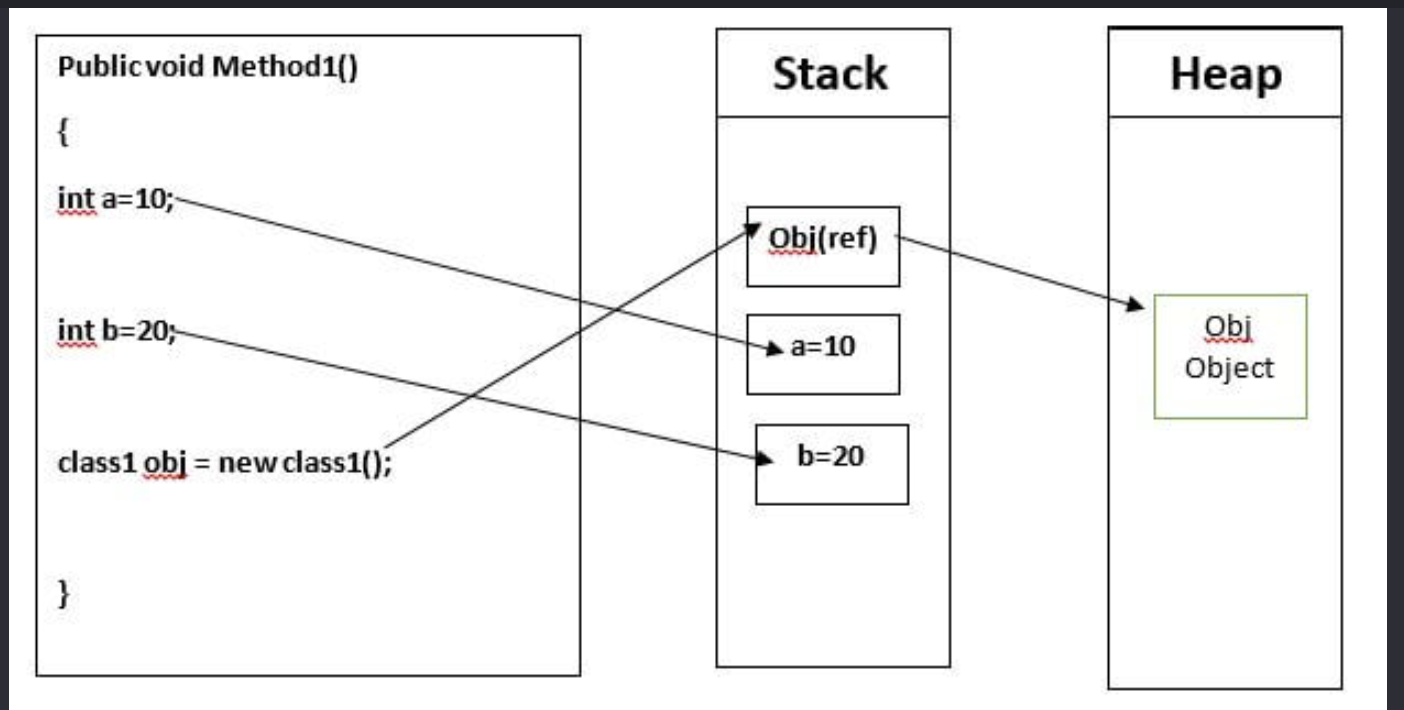
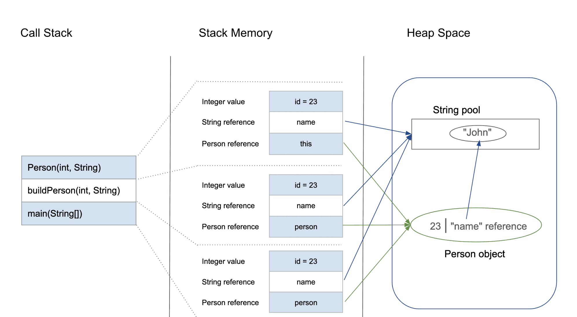
Stack and heap

Now we reach another important concept.

A running program uses memory in different ways. Two areas you’ll encounter immediately are the stack and the heap.

Consider:

void calculate() {
int number = 42;
}

The local variable has automatic storage associated with the function’s execution.

Conceptually:

Stack
calculate()
┌───────────────┐
│ number = 42 │
└───────────────┘

When the function returns, that stack storage is no longer needed.

Dynamic allocation is different:

int *number = malloc(sizeof(int));
*number = 42;

Now memory is allocated dynamically.

Conceptually:

Stack
┌───────────────┐
│ number │──────┐
└───────────────┘ │
↓
Heap
┌────────┐
│ 42 │
└────────┘

And C expects you to eventually release it:

free(number);

This explicit ownership model is one of the biggest differences between C and Ruby.

C always need to know, how large a piece of data is and where do I put it. Everything in C is something like: name + address + value


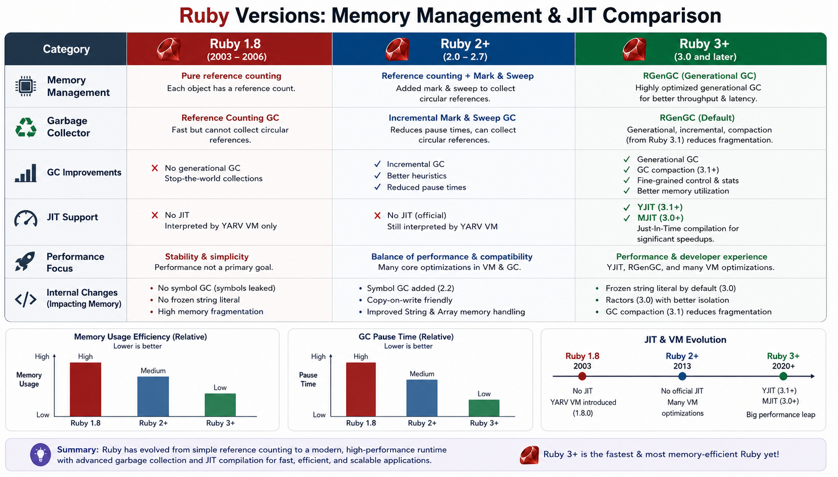
Ruby Memory Management – JIT Comparision

Check: https://docs.ruby-lang.org/en/3.4/yjit/yjit_md.html


Ruby’s heap becomes a much more interesting subject

In Ruby, you normally write:

user = User.new

and never ask:

Who called malloc?
Where exactly is this object?
Who will release its memory?

Ruby’s runtime manages those details.

The object is allocated under Ruby’s memory-management system and the garbage collector tracks object reachability and determines when memory can be reclaimed.

So rather than:

Application → malloc → free

you generally experience:

Ruby code
↓
Ruby runtime
↓
allocation
↓
Ruby heap
↓
GC

Learning C makes that second model much easier to reason about.


The fascinating part: VALUE

Now we arrive at one of the concepts that makes CRuby internals especially interesting.

In CRuby, Ruby values are represented internally using a type called:

VALUE

You will encounter VALUE everywhere when reading the Ruby C implementation and C extension APIs.

Conceptually, you can think of it as:

the low-level representation Ruby uses to pass around Ruby values inside the runtime.

For example, a Ruby C API function may look conceptually like:

VALUE rb_str_new_cstr(const char *ptr);

and C extension methods often receive and return VALUEs.

That means your Ruby object:

"hello"

does not remain some abstract concept all the way down.

CRuby represents it using its internal object/value machinery.


Not every Ruby value is simply a pointer

This is where Ruby becomes particularly interesting.

A common beginner assumption is:

Ruby object = pointer to heap object

That’s useful as a rough mental model, but it isn’t the whole story.

CRuby uses a representation that can encode certain immediate values directly rather than allocating a separate heap object for every value.

Integers are a classic example.

So when you write:

number = 42

you shouldn’t automatically imagine:

number
↓
heap object containing 42

The runtime has specialized representations for some Ruby values.

This is one reason looking at CRuby internals is so educational.

A high-level statement such as:

“Ruby variables point to objects”

is useful, but the implementation is much more nuanced.


Why this matters for a Ruby developer

Let’s take:

a = 10
b = 10

At the Ruby language level, you care that both variables represent the integer 10.

After learning some C and Ruby internals, you start asking different questions:

Are these separate objects?
Is 10 heap allocated?
How does CRuby represent integers?
How does Ruby distinguish integers from ordinary heap objects?
What exactly is stored in VALUE?

Those are much deeper questions.

And they lead directly into:

  • immediate values
  • object flags
  • object headers
  • pointer tagging
  • garbage collection
  • object allocation
  • Ruby’s internal data structures

Pointers explain something else: object identity

Ruby lets us ask:

a = Object.new
b = a
a.equal?(b)
# => true

Why?

Because both variables refer to the same object.

Conceptually:

a ─────┐
↓
[Object]
↑
│
b ─────┘

C gives you the vocabulary to understand this relationship:

reference
address
pointer
memory location

Again, Ruby intentionally hides the actual pointer from application code.

But the underlying concept of “multiple references to the same object” remains.


The danger of C is also the lesson

Ruby protects you from many classes of memory errors.

In C, you can easily write:

int *ptr = malloc(sizeof(int));
*ptr = 42;
free(ptr);
*ptr = 100;

Now you’re accessing memory after it has been released.

That’s a use-after-free.

You can also leak memory:

int *ptr = malloc(sizeof(int));
/* forgot free(ptr) */

Or write outside an allocated buffer:

int numbers[10];
numbers[100] = 42;

These bugs are difficult precisely because C gives you so much control.

And that is the paradox:

The freedom that makes C powerful is the same freedom that makes it dangerous.

Ruby takes many of these responsibilities away from you.


The real payoff

After learning these concepts, this Ruby code:

users = 10_000.times.map { User.new }

starts looking different.

Instead of only seeing:

Ruby objects

you can begin thinking:

Ruby objects
↓
object representation
↓
memory allocation
↓
references
↓
Ruby heap
↓
garbage collector

And when a Rails application starts consuming hundreds of megabytes of memory, that mental model becomes much more useful.

You can ask better questions.

Not just:

“Why is Rails using so much memory?”

but:

“What objects are being allocated, how long do they remain reachable, and how does Ruby’s allocator and GC interact with that workload?”

That’s a much more senior-level way of investigating the problem.


Where we go next

We have now established the foundation:

C
↓
Memory
↓
Addresses
↓
Pointers
↓
Stack / Heap
↓
Ruby references
↓
VALUE
↓
CRuby object representation

The next step gets even more interesting:

What does a Ruby object actually look like inside CRuby?

We’ll look at concepts such as object headers, RBasic, type information, flags, heap allocation, and how the garbage collector sees Ruby objects.

That’s where the gap between:

User.new

and:

VALUE obj;

starts to disappear.

Happy Learning! 🚀

Learning C to Understand Ruby: A Senior Ruby Developer’s Journey – Part 1

As a Ruby developer, I have spent years enjoying one of Ruby’s biggest strengths: abstraction.

In Rails, I can write:

users = User.where(active: true)

and focus on the business problem rather than memory allocation, pointers, system calls or CPU instructions.

That is exactly why Ruby is productive.

But recently, I started asking a different question:

What is actually happening underneath my Ruby code?

What happens when Ruby creates an object?
Where does that object live?
Who allocates the memory?
Who releases it?
What does an array really look like internally?
What happens when Ruby calls a method?

And that leads to an interesting realization:

Learning C is not necessarily about moving away from Ruby. It can be a way of understanding Ruby at a much deeper level.

This is the first part of that journey.


Ruby hides the machine – intentionally

Consider this:

user = User.new

At the Ruby level, this is trivial.

But conceptually, a lot more is happening.

Ruby needs to:

  1. Represent the object.
  2. Allocate memory for it.
  3. Initialize its internal state.
  4. Keep track of the object for garbage collection.
  5. Maintain references between objects.
  6. Eventually reclaim its memory.

Ruby handles these details for us.

That abstraction is one of the reasons we love Ruby.

But it also means that most Ruby developers don’t need to think about the actual machine.

C removes much of that abstraction.


C forces you to think about memory

In C, you quickly encounter things like:

int number = 42;

and:

int *ptr = &number;

The second line introduces a concept that Ruby normally keeps away from you: the memory address of a value.

You can explicitly allocate memory:

int *numbers = malloc(100 * sizeof(int));

and explicitly release it:

free(numbers);

That changes your mental model.

Instead of thinking only in terms of:

objects
methods
classes

you begin thinking about:

memory
addresses
bytes
layouts
allocation
lifetime
references

And this is extremely useful when trying to understand Ruby internally.


Ruby objects are still data in memory

Take a simple Ruby value:

name = "Abhilash"

As a Ruby developer, you normally think:

name → String

A lower-level mindset makes you ask:

name
  ↓
Ruby value/reference
  ↓
Object representation
  ↓
Memory
  ↓
Bytes

Ruby doesn’t magically escape the laws of computing.

At some point, that string has to exist in memory.

The same is true for:

Array
Hash
Integer
String
User

They all ultimately have machine-level representations.

Learning C helps you become curious about those representations.


Stack vs Heap

One of the first concepts worth learning in C is the difference between stack and heap memory.

For example:

void example() {
    int number = 10;
}

The local variable has automatic storage duration associated with the function’s execution.

Dynamic allocation looks different:

int *number = malloc(sizeof(int));
*number = 10;

free(number);

Now the program explicitly controls the allocation and lifetime.

This distinction is extremely important when later studying Ruby’s memory management.

Ruby objects are managed by the runtime rather than by application code using malloc and free directly.

That leads naturally to the next question:

Who manages Ruby’s heap?

The answer takes us into the Ruby garbage collector.


Garbage collection becomes much easier to understand

A Ruby developer typically learns:

“Ruby has a garbage collector, so I don’t need to manually free objects.”

That’s correct, but incomplete.

Once you understand manual memory management in C, garbage collection becomes much more interesting.

You can start thinking about:

Object allocation
       ↓
Heap
       ↓
References
       ↓
Object becomes unreachable
       ↓
Garbage collector
       ↓
Memory can be reclaimed

Instead of viewing GC as some magical Ruby feature, you begin seeing it as a runtime memory-management strategy.

That distinction is important.

Ruby didn’t eliminate memory management.

It automated memory management.


C also teaches you that data layout matters

Consider:

struct User {
    int id;
    char name[50];
};

You are explicitly describing a data structure’s layout.

You begin thinking about questions such as:

  • How many bytes does this structure occupy?
  • How are fields aligned?
  • Are objects contiguous?
  • How efficiently will the CPU access them?
  • What happens to cache locality?

Ruby normally shields you from these concerns.

But when performance suddenly matters, these concepts become valuable.

For example, processing millions of objects isn’t only about algorithmic complexity.

Memory access patterns can matter too.

This is one reason understanding low-level systems concepts can make you a better high-level developer.


Then there is the most interesting part: Ruby itself uses C

This is where the journey becomes particularly relevant to Ruby developers.

The standard Ruby implementation, CRuby, is largely implemented in C.

That means the language we write:

array.map(&:name)

eventually reaches a runtime implemented at a much lower level.

Conceptually:

Ruby code
   ↓
Ruby parser / VM
   ↓
CRuby runtime
   ↓
Operating system
   ↓
CPU / memory

Once you start reading Ruby’s C source code, concepts that initially look mysterious start becoming understandable:

VALUE
Ruby objects
references
object allocation
method dispatch
garbage collection
VM execution

And suddenly C stops being just another programming language.

It becomes a lens through which you can inspect Ruby itself.


Why should a senior Rails developer care?

You don’t need to write your next Rails application in C.

That isn’t the point.

The goal is to develop a deeper mental model.

When you write:

100_000.times do
User.new
end

you should eventually be able to think beyond the Ruby syntax.

You start wondering:

How many allocations?

Where are those objects stored?

How does GC discover them?

What references exist?

How much memory is being consumed?

What happens when these objects become unreachable?

What is the runtime doing while my Ruby code executes?

Those questions are far more valuable than memorizing another Rails API.


The goal of this journey

My objective isn’t:

“Become a C programmer.”

It is:

Become a Ruby developer who understands what Ruby is doing underneath.

And the roadmap becomes surprisingly clear:

C fundamentals
      ↓
Pointers & memory
      ↓
Stack & heap
      ↓
Processes & system calls
      ↓
C programming at system level
      ↓
CRuby internals
      ↓
Ruby VM
      ↓
Garbage collection
      ↓
Ruby C extensions

The interesting part is that the deeper you go into C, the less mysterious Ruby becomes.

Ruby’s abstractions don’t disappear.

You simply start seeing what is behind them.

And for me, that is the real power of learning C as a Ruby developer.

Part 2 will start with the most important foundation: memory, pointers, stack, heap and how these concepts map to the Ruby object model.

For Part 2, I’d make memory + pointers + stack/heap → Ruby objects. That is where this series can become genuinely fascinating for an experienced Ruby developer.

Happy Learning! 🚀

The Magic of +”” and -“” in Ruby

Demystifying Unary String Operators for Performance and Safety

Ruby is renowned for its developer happiness and elegant syntax. It’s a language where common tasks often read like natural English. However, beneath this friendly surface lie powerful, slightly esoteric features designed for fine-grained control and performance optimization. One such feature – often puzzling to newcomers and occasionally overlooked by seasoned developers – is the use of unary operators on strings: specifically, +”” and -“” .

If you’ve ever dug into the source code of popular Ruby gems like Rails or sidekiq, you might have stumbled across a line like this and paused:

buffer = +""

What exactly is happening here? Why not just write buffer = “” ? Let’s dive into the mechanics, the advantages, and why this tiny symbol makes a significant difference.

The Problem: The Frozen String Literal Pragma

To understand +”” , we first have to understand a major shift in Ruby’s approach to memory management.

Historically, every time you declared a string literal in Ruby, a new object was created in memory. If you had a loop that printed “hello” 1,000 times, Ruby instantiated 1,000 distinct string objects, creating work for the garbage collector.
To combat this, Ruby 2.3 introduced the frozen string literal pragma:

frozen_string_literal: true

When placed at the top of a file, this magic comment instructs Ruby to freeze all string literals in that file. A frozen string cannot be modified. They become constants in memory, drastically reducing object allocations. This is considered a best practice in modern Ruby development.

However, this introduces a new problem. What if you want to build a string dynamically using append operations ( << )?

frozen_string_literal: true
buffer = ""
buffer << "Hello" # => FrozenError (can't modify frozen String)

The Solution: The Unary Plus ( +”” )

Enter the unary + operator. Introduced in Ruby 2.3 alongside the frozen string pragma, + explicitly unfreezes a string literal, returning a mutable copy.

frozen_string_literal: true
buffer = +""
buffer << "Hello "
buffer << "World"
puts buffer # => "Hello World"

In short: +”” says to Ruby, “I know frozen strings are enabled here, but I specifically need this particular string to be mutable because I plan to change it.”

Why is this better than String.new ?

You could achieve the same result using String.new .

buffer = String.new

Functionally, +”” and String.new achieve the same goal. However, +”” is generally preferred in the Ruby community for a few reasons:
* Brevity: It’s significantly shorter and reads more like a literal assignment.
* Idiomatic: It has become the recognized standard idiom in modern Ruby libraries.
* Performance (Micro-optimization): Historically, evaluating the literal +”” was marginally faster than the method dispatch required for String.new , although modern Ruby versions have largely leveled this playing field.

The Counterpart: The Unary Minus ( -“” )

If + unfreezes a string, what does – do? The unary minus does the opposite: it
guarantees a string is frozen and deduplicated.

frozen_string_literal: false (or omitted)
str1 = -"immutable"
str2 = -"immutable"
puts str1.object_id == str2.object_id # => true
str1 << " change" # => FrozenError (can't modify frozen String)

When you use – , Ruby checks an internal “frozestring” table. If a frozen string with the identical content already exists, it returns a reference to that existing object rather than creating a new one. This is equivalent to calling “immutable”.freeze , but it is syntactically cleaner when used inline.

Why Do Developers Miss This?

If these operators are so useful, why aren’t they universally understood?
* It’s visually subtle: The difference between “” and +”” is a single character. It’s easy for the eyes to glide over it during code review or while casually reading a library’s source code.
* It relies on file-level pragmas: If you aren’t in the habit of using #
frozen_string_literal: true
in your projects, you rarely encounter the
FrozenError that necessitates +”” . Many smaller scripts or older legacy
applications run without the pragma, meaning a regular “” works fine as a
mutable buffer.
* It feels “un-Ruby-like”: Ruby is usually explicit and readable (e.g., [1,
2].empty? ). Using arithmetic operators like + and – on strings to control memory allocation feels a bit like C-style pointer manipulation, which breaks the mental model some developers have of the language.

Best Practices & Takeaways

To write modern, performant, and safe Ruby code, adopt these habits:
* Always freeze by default: Add # frozen_string_literal: true to the top of all new Ruby files. It’s an easy win for memory efficiency.
* Use +”” for buffers: When you need to incrementally build a string using << ,
initialize it with +”” .
* Avoid += in loops: Building strings with += creates a new object on every iteration, regardless of pragmas. Always prefer appending to a mutable buffer with << .

BAD (Creates 1001 string objects)
frozen_string_literal: true
result = +""
1000.times { result += "a" }
GOOD (Creates 1 mutable string object and modifies it in place)
frozen_string_literal: true
result = +""
1000.times { result << "a" }

The unary operators + and – on strings are small, esoteric features that pack a
significant punch. Understanding them not only helps you write better code but also enables you to read and understand the source code of the Ruby ecosystem’s most robust libraries.

Files

Download PDF:

Happy Rubying!

Learn SQL: Day 7 – Query Optimization Workshop

Welcome to Day 7.

Everything we’ve learned so far leads to this lesson.

Until now, you’ve learned:

  • How to write SQL
  • How JOINs work
  • How GROUP BY works
  • How indexes work
  • How PostgreSQL chooses execution plans

Today, we’ll combine everything to solve real-world performance problems.


Today’s Goals

By the end of today, you’ll be able to answer questions like:

  • Why is this query slow?
  • Should I add an index?
  • Should I rewrite the query?
  • Is this a database problem or an application problem?
  • How would I debug this in production?

These are exactly the kinds of discussions that happen in senior Rails interviews.


A Senior Engineer’s Workflow

Suppose your manager says:

“The Users page takes 8 seconds to load.”

A junior developer might immediately say:

“Let’s add an index.”

A senior developer thinks:

1. Is the query actually slow?
2. Which query is slow?
3. How much data is involved?
4. What is PostgreSQL doing?
5. Can I rewrite the query?
6. Do I need an index?
7. Is the application causing the problem?

Notice:

Adding an index is Step 6, not Step 1.

Our Practice Schema

Let’s build something closer to a real Rails application.

DROP TABLE IF EXISTS order_items;
DROP TABLE IF EXISTS orders;
DROP TABLE IF EXISTS products;
DROP TABLE IF EXISTS users;

Users

CREATE TABLE users (
    id BIGSERIAL PRIMARY KEY,
    name TEXT,
    email TEXT,
    city TEXT
);

Products

CREATE TABLE products (
    id BIGSERIAL PRIMARY KEY,
    name TEXT,
    price NUMERIC(10,2),
    category TEXT
);

Orders

CREATE TABLE orders (
    id BIGSERIAL PRIMARY KEY,
    user_id BIGINT NOT NULL REFERENCES users(id),
    status TEXT,
    created_at TIMESTAMP DEFAULT NOW()
);

Order Items

CREATE TABLE order_items (
    id BIGSERIAL PRIMARY KEY,
    order_id BIGINT NOT NULL REFERENCES orders(id),
    product_id BIGINT NOT NULL REFERENCES products(id),
    quantity INTEGER,
    price NUMERIC(10,2)
);


The Six-Step Performance Checklist

Every slow query investigation should start with this checklist.

Step 1 – Measure

Never optimise blindly.

Run:

EXPLAIN ANALYZE
SELECT ...

Step 2 – Understand the Business Question

Example:

Show the last 20 completed orders.

Don’t optimise before understanding what the query should do.

Step 3 – Read the Plan

Look for:

  • Seq Scan
  • Nested Loop
  • Hash Join
  • Sort
  • Aggregate
  • Bitmap Heap Scan

Step 4 – Find the Bottleneck

Ask:

  • Which node took the most time?
  • Which node processed the most rows?

Step 5 – Decide the Fix

Possible fixes:

  • Better index
  • Better SQL
  • Better schema
  • Better ActiveRecord
  • Better pagination

Step 6 – Measure Again

Never assume the optimisation worked.

Always compare before and after.


Scenario 1 – Missing Index

Query:

SELECT *
FROM users
WHERE email='john@example.com';

Execution plan:

Seq Scan
rows=100000
actual rows=1

Question:

What’s wrong?

Diagnosis

No index on email.

Fix

CREATE INDEX idx_users_email
ON users(email);

Run again:

EXPLAIN ANALYZE
SELECT *
FROM users
WHERE email='john@example.com';

Expect:

Index Scan

Scenario 2 – Wrong Index

Suppose the application runs:

SELECT *
FROM users
WHERE city='Chicago'
AND age=30;

Indexes:

(city)
(age)

Question:

Better solution?

Answer

Composite index:

CREATE INDEX idx_city_age
ON users(city, age);

Because the application almost always filters by both.


Scenario 3 – Sorting

Query:

SELECT *
FROM orders
ORDER BY created_at DESC
LIMIT 20;

Plan:

Seq Scan
↓
Sort
↓
Limit

Question:

Can we avoid sorting?

Solution

CREATE INDEX idx_orders_created_at_desc
ON orders(created_at DESC);

Now PostgreSQL can read the index in order.

Often:

Index Scan
↓
Limit

No Sort node.


Scenario 4 – N+1 Queries

Rails code:

orders = Order.limit(100)

orders.each do |order|
  puts order.user.name
end

SQL executed:

SELECT * FROM orders LIMIT 100;

Then:

SELECT * FROM users WHERE id=1;

SELECT * FROM users WHERE id=2;

…

100 additional queries.

Total

101 queries

Fix

Order.includes(:user)

Now:

SELECT * FROM orders;
SELECT *
FROM users
WHERE id IN (...);

Two queries.

Interview Question

Which is faster?

includes

or

joins

Answer:

They solve different problems.


Scenario 5 – OFFSET Pagination

Query:

SELECT *
FROM orders
ORDER BY created_at DESC
LIMIT 20
OFFSET 100000;

Looks harmless.

But PostgreSQL must skip:

100000 rows

before returning:

20 rows

Large OFFSET values become increasingly expensive.

Better Solution

Keyset Pagination.

Instead of:

OFFSET 100000

Use:

WHERE created_at < '2026-07-01'
ORDER BY created_at DESC
LIMIT 20;

This lets PostgreSQL continue from the last seen row instead of counting through earlier rows.

Rails Example

Instead of:

Order.order(created_at: :desc)
     .offset(100000)
     .limit(20)

Use:

Order
  .where("created_at < ?", last_created_at)
  .order(created_at: :desc)
  .limit(20)

This is called keyset pagination or cursor pagination.


Scenario 6 – SELECT *

Query:

SELECT *
FROM users;

Returns:

id
name
email
city
address
bio
avatar
...

Suppose the page only displays:

  • name
  • city

Why fetch everything?

Better:

SELECT
name,
city
FROM users;

Rails:

User.select(:name, :city)

Scenario 7 – COUNT(*)

Suppose:

SELECT COUNT(*)
FROM orders;

On:

300 million rows

Question:

Can this be slow?

Yes.

Because PostgreSQL must count visible rows.

Unlike some databases, PostgreSQL generally doesn’t maintain an exact row count that’s instantly available for arbitrary COUNT(*).


Scenario 8 – DISTINCT

Query:

SELECT DISTINCT users.*
FROM users
JOIN orders
ON users.id=orders.user_id;

Question:

Why is DISTINCT needed?

Because JOIN duplicates users.

Could EXISTS express the requirement more directly?

SELECT *
FROM users u
WHERE EXISTS (
SELECT 1
FROM orders o
WHERE o.user_id=u.id
);

Sometimes that’s clearer.


Scenario 9 – Functions in WHERE

Query:

SELECT *
FROM users
WHERE LOWER(email)='john@example.com';

Normal email index?

Not useful.

Solution:

CREATE INDEX idx_lower_email
ON users(LOWER(email));

Expression index.


Scenario 10 – Too Many Indexes

Suppose:

users
↓
12 indexes

Problem?

Every INSERT must update:

Table
+
12 indexes

Indexes speed reads but slow writes.

Always consider the workload.


Optimization Decision Tree

When a query is slow, ask:

Is PostgreSQL scanning too many rows?
│
▼
Yes
│
▼
Would an index help?
│
▼
Yes
│
▼
Do I already have one?
│
▼
No
│
▼
Create the correct index.

But also ask:

Am I returning unnecessary data?
Am I sorting unnecessarily?
Am I joining unnecessarily?
Am I executing the query too many times?

Real Rails Optimization Example

Suppose this page loads slowly:

@orders = Order
            .where(status: "completed")
            .order(created_at: :desc)
            .limit(20)

Questions:

  1. Is there an index on status?
  2. Is there an index on created_at?
  3. Would a composite index help?

Potential solution:

CREATE INDEX idx_orders_status_created_at
ON orders(status, created_at DESC);

Why?

Because the query filters by status and orders by created_at.


Senior Interview Exercise

Suppose you see:

SELECT *
FROM orders
WHERE user_id = 100
ORDER BY created_at DESC
LIMIT 20;

Which index would you create?

Many people answer:

(user_id)
(created_at)

A stronger answer is:

CREATE INDEX idx_orders_user_created
ON orders(user_id, created_at DESC);

Because it supports both the filter and the ordering in one index.


Common Performance Mistakes

Mistake 1

Adding indexes without measuring.

Mistake 2

Using SELECT * everywhere.

Mistake 3

Ignoring N+1 queries.

Mistake 4

Using huge OFFSET values.

Mistake 5

Creating duplicate indexes.

Mistake 6

Ignoring EXPLAIN ANALYZE.

Senior-Level Mental Model

Every query has a “cost.”

The cost comes from:

Rows read
+
Rows sorted
+
Rows joined
+
Rows transferred
+
Application round trips

The goal of optimisation is to reduce one or more of these.


Practical Exercises

Exercise 1

Create:

CREATE INDEX idx_orders_user_created
ON orders(user_id, created_at DESC);

Run:

EXPLAIN ANALYZE
SELECT *
FROM orders
WHERE user_id=1
ORDER BY created_at DESC
LIMIT 20;

Observe whether PostgreSQL can avoid an explicit Sort.

Exercise 2

Compare:

SELECT *
FROM users;

with:

SELECT name, city
FROM users;

Think about the amount of data returned.

Exercise 3

Write three versions of:

“Find users with completed orders.”

Using:

  1. JOIN
  2. EXISTS
  3. IN

Then compare their execution plans.

Exercise 4

Find a query that performs a Seq Scan.

Add an appropriate index.

Run EXPLAIN ANALYZE again.

What changed?


Interview Case Study

Imagine you’re in a senior Rails interview.

The interviewer says:

“A customer reports that the Orders page takes 6 seconds to load.”

A strong answer isn’t:

“I’ll add an index.”

A stronger answer is:

  1. Reproduce the issue.
  2. Identify the SQL generated by ActiveRecord.
  3. Run EXPLAIN ANALYZE.
  4. Inspect scan types, joins, and sort operations.
  5. Check existing indexes.
  6. Decide whether the fix belongs in the SQL, indexes, ActiveRecord code, or schema.
  7. Measure again after the change.

That systematic approach demonstrates senior-level thinking.


Homework

Build a small benchmark using your practice schema.

  1. Populate:
    • 100,000 users
    • 500,000 orders
  2. Measure these queries before and after adding indexes:
    • Find a user by email.
    • Find recent orders for a user.
    • Find completed orders.
    • Find users with no orders.
  3. For each query, record:
    • Execution plan
    • Execution time
    • Scan type
    • Rows estimated
    • Rows returned
  4. Explain why PostgreSQL chose each plan.

What’s Next?

At this point, you’re already covering topics that many experienced Rails developers never study in depth.

For Day 8, I recommend Window Functions:

  • ROW_NUMBER()
  • RANK()
  • DENSE_RANK()
  • LAG()
  • LEAD()
  • Running totals
  • Moving averages
  • Top N per group

Window functions are common in reporting, analytics, and senior backend interviews because they solve problems that are difficult or inefficient with plain GROUP BY. Understanding them will significantly broaden your SQL toolkit.

Happy Learning! 🚀

Learn SQL: Day 6C – Mastering EXPLAIN ANALYZE (Think Like the PostgreSQL Query Planner)

Welcome to Day 6C.

This is one of the most valuable lessons in the entire course.

Many developers know how to write SQL.

Very few can answer questions like:

“Why is this query slow?”

or

“Why did PostgreSQL choose a Bitmap Heap Scan instead of an Index Scan?”

or

“What would you optimize first?”

This lesson will teach you exactly that.

Today’s Goal

By the end of today, you should be able to:

  • Read an EXPLAIN ANALYZE plan from top to bottom
  • Understand every important field
  • Explain why PostgreSQL chose a plan
  • Identify bottlenecks
  • Suggest optimizations
  • Discuss execution plans confidently in a senior interview

First, Understand What EXPLAIN ANALYZE Actually Does

Consider this query:

SELECT *
FROM users
WHERE email = 'user50000@example.com';

Without EXPLAIN, PostgreSQL simply returns the result.

With:

EXPLAIN
SELECT *
FROM users
WHERE email = 'user50000@example.com';

PostgreSQL says:

“Here’s the plan I intend to use.”

With:

EXPLAIN ANALYZE
SELECT *
FROM users
WHERE email = 'user50000@example.com';

PostgreSQL actually executes the query and says:

“Here’s what really happened.”

The Query Planner

Imagine PostgreSQL as a GPS.

You ask:

Go from A to B.

The GPS considers:

  • Highway
  • Local roads
  • Toll roads
  • Traffic

Then chooses the cheapest route.

PostgreSQL does exactly the same.

It considers:

  • Sequential Scan
  • Index Scan
  • Bitmap Scan
  • Hash Join
  • Nested Loop
  • Merge Join

and chooses what it estimates to be the cheapest plan.

Our Practice Table

Use the same table from Day 6B.

users

100,000 rows.

Our First Plan

EXPLAIN ANALYZE
SELECT *
FROM users
WHERE email='user50000@example.com';

You might see something similar to:

Index Scan using idx_users_email on users
(cost=0.42..8.44 rows=1 width=51)
(actual time=0.030..0.032 rows=1 loops=1)

Let’s decode every part.


Part 1 – Scan Type

First line:

Index Scan

This answers:

How did PostgreSQL access the table?

Possible answers:

  • Seq Scan
  • Index Scan
  • Index Only Scan
  • Bitmap Heap Scan

The scan type is the first thing you should notice.


Part 2 – Using Which Index?

using idx_users_email

PostgreSQL tells you exactly which index it used.

If you expected:

idx_users_city

but it chose:

idx_users_age

you should ask yourself why.


Part 3 – Cost

Example:

cost=0.42..8.44

Many beginners think:

“8.44 milliseconds.”

No.

Cost is not time.

It is PostgreSQL’s internal scoring system.

Think of it like this:

Plan A
Cost = 150
Plan B
Cost = 70

PostgreSQL chooses Plan B.

Startup Cost

First number:

0.42

Cost before the first row can be returned.

Total Cost

Second number:

8.44

Cost to return every row.


Part 4 – Rows

rows=1

Planner estimate.

Meaning:

"I think this query will return
1 row."

Part 5 – Width

width=51

Estimated average size of one returned row.

Used internally for memory and I/O estimates.


Part 6 – Actual Time

actual time=0.030..0.032

Meaning:

First row
↓
0.030 ms

Entire query finished:

0.032 ms

Part 7 – Actual Rows

actual rows=1

Excellent.

Planner guessed:

1

Reality:

1

Very accurate.


Part 8 – Loops

loops=1

This operation executed once.

You’ll later see plans like:

loops=100000

That often indicates an expensive nested loop.


Reading Plans from Bottom to Top

This surprises many developers.

Execution plans are printed like a tree.

Example:

Limit
↓
Sort
↓
Index Scan

Although Limit appears first, execution begins at the bottom.

Conceptually:

Index Scan
↓
Sort
↓
Limit

Think of a factory:

Raw Material
↓
Machine 1
↓
Machine 2
↓
Finished Product

The raw material starts at the bottom.


Example 2 – Sequential Scan

EXPLAIN ANALYZE
SELECT *
FROM users
WHERE city='Chicago';

Output:

Seq Scan on users
(cost=0.00..2332.00 rows=24780 width=51)
(actual time=0.08..21.10 rows=25000 loops=1)

Let’s interpret it.

Why Seq Scan?

Question:

How many rows match?

25,000

That’s:

25%

of the table.

Using the index might require:

  • index lookup
  • 25,000 table lookups

Sequential Scan may simply be cheaper.

Interview Question

If PostgreSQL ignores your index,

does that mean

the index is useless?

Answer:

Absolutely not.

It means PostgreSQL estimated another plan to be cheaper for that specific query.


Example 3 – Bitmap Heap Scan

Suppose you create:

CREATE INDEX idx_users_city
ON users(city);

Now:

EXPLAIN ANALYZE
SELECT *
FROM users
WHERE city='Chicago';

Output:

Bitmap Heap Scan
↓
Bitmap Index Scan

Notice there are two nodes.

Bitmap Index Scan

First:

Read the index.

Chicago
↓
Rows
4
8
12
...

Bitmap Heap Scan

Then:

Visit the table efficiently.

Instead of:

Index
↓
Table
↓
Index
↓
Table

It does:

Index
↓
Collect row locations
↓
Read pages together

Excellent for medium-sized result sets.

Visual

Bitmap Index Scan
↓
Matching Row IDs
↓
Bitmap Heap Scan
↓
Actual Rows

Example 4 – Index Only Scan

Suppose:

SELECT email
FROM users
WHERE email='user100@example.com';

Plan:

Index Only Scan

Question:

Why is this faster?

Answer:

Because PostgreSQL answered the query using only the index.

No table lookup.

Planning Time vs Execution Time

Example:

Planning Time: 0.2 ms
Execution Time: 0.3 ms

Planning:

Choosing the route.

Execution:

Driving the route.

Why Estimates Matter

Suppose:

Planner:

rows=5

Reality:

actual rows=50000

Huge difference.

The planner may choose a terrible plan because its estimate was wrong.

This usually indicates stale statistics.

ANALYZE

Run:

ANALYZE users;

PostgreSQL updates statistics.

The planner now has better information.

VACUUM ANALYZE

Often you’ll see:

VACUUM ANALYZE users;

It does two things:

  • Cleans dead tuples
  • Updates statistics

We’ll study MVCC later.

The Most Common Plan Nodes

These are the ones you should know well for interviews.

Seq Scan

Reads every row.

Think:

Read entire book.

Index Scan

Uses an index.

Think:

Use the book's index.

Index Only Scan

Never touches the table.

Think:

Everything I need is already in the index.

Bitmap Index Scan

Collect matching row locations.

Bitmap Heap Scan

Fetch those rows efficiently.

Sort

ORDER BY

often produces:

Sort

Sorting millions of rows can be expensive.

Aggregate

Produced by:

COUNT()
SUM()
AVG()
GROUP BY

Hash Join

Often used for joins.

We’ll study joins from PostgreSQL’s perspective soon.

Nested Loop

Good when:

One side is tiny.

Terrible when:

Both sides are huge.

Limit

Produced by:

LIMIT 10

Real Example

SELECT *
FROM users
ORDER BY created_at DESC
LIMIT 10;

Possible plan:

Limit
↓
Sort
↓
Seq Scan

Question:

Can we improve it?

Yes.

Index:

CREATE INDEX idx_created_at
ON users(created_at DESC);

Now PostgreSQL may avoid sorting completely.

Buffers (Advanced)

Sometimes you’ll see:

Buffers:
shared hit=500
read=2

Meaning:

Most pages were already in memory.

We’ll study this later.

Parallel Query

Sometimes:

Gather
↓
Parallel Seq Scan

PostgreSQL used multiple CPU workers.

Very common for huge tables.

How to Read Any Plan

I use this checklist.

Step 1

What is the scan type?

Step 2

Which index?

Step 3

Estimated rows?

Step 4

Actual rows?

Step 5

Huge mismatch?

If yes,

statistics may be wrong.

Step 6

Planning vs execution time.

Step 7

Which operation consumed most of the cost?


Real Interview Example

Interviewer shows:

Seq Scan
rows=100000
actual rows=1

Question:

Would you optimize?

Yes.

Probably missing an index.

Another example:

Index Scan
rows=90000

Question:

Should PostgreSQL maybe use Seq Scan?

Possibly.

Need to inspect the query.


Common Mistakes

Mistake 1

Thinking cost is milliseconds.

Wrong.

Mistake 2

Looking only at execution time.

Also inspect:

  • estimated rows
  • actual rows

Mistake 3

Ignoring scan type.

Always notice:

Seq
Index
Bitmap
Index Only

Mistake 4

Assuming an index must always be used.

False.

Senior-Level Interview Questions

Q1

Difference:

EXPLAIN
EXPLAIN ANALYZE

Q2

Why can PostgreSQL ignore an index?

Q3

What does

rows

mean?

Q4

Difference between

rows
actual rows

Q5

What is

loops

?

Q6

Difference between

Index Scan
Index Only Scan

Q7

Why is Bitmap Heap Scan useful?

Q8

Why isn’t cost measured in milliseconds?

Q9

How do stale statistics affect query plans?

Q10

Why should you run

ANALYZE

after major data changes?


Practical Exercises

Exercise 1

Run:

EXPLAIN ANALYZE
SELECT *
FROM users
WHERE email='user50000@example.com';

Write down:

  • Scan type
  • Estimated rows
  • Actual rows
  • Execution time

Exercise 2

Run:

EXPLAIN ANALYZE
SELECT *
FROM users
WHERE city='Chicago';

Explain why PostgreSQL chose that plan.

Exercise 3

Run:

EXPLAIN ANALYZE
SELECT *
FROM users
ORDER BY created_at DESC
LIMIT 10;

Then create an index:

CREATE INDEX idx_users_created_at_desc
ON users(created_at DESC);

Run the query again and compare the plans.

Exercise 4

Run:

ANALYZE users;

Then compare the estimated rows with the actual rows again.


Senior Rails Interview Tips

If an interviewer gives you an execution plan, don’t immediately suggest adding an index.

Instead, ask:

  1. How many rows are in the table?
  2. How many rows does this query return?
  3. What indexes already exist?
  4. Is the planner’s estimate accurate?
  5. Is the query actually slow?

That line of reasoning demonstrates experience much better than jumping straight to “add an index.”


What’s Next?

From here, I recommend Day 7: Query Optimization Workshop.

Unlike the previous lessons, it won’t introduce many new SQL keywords. Instead, we’ll work through real production-style problems, such as:

  • A query that takes 8 seconds—how do we optimize it?
  • Why did PostgreSQL choose a Nested Loop instead of a Hash Join?
  • N+1 queries in Rails and how to eliminate them.
  • OFFSET pagination vs keyset pagination.
  • Rewriting slow SQL into faster SQL.
  • Using indexes effectively rather than adding them blindly.

This is the stage where you’ll start thinking like a senior backend engineer rather than someone who simply knows SQL syntax.

Happy Learning! 🚀

Learn SQL: Day 6B – Advanced Indexing (Senior-Level Insights)

Welcome to Day 6B.

Today we’ll go beyond “create an index” and learn how senior backend engineers decide which index to create.

This is one of the most valuable topics for PostgreSQL and Rails interviews.

By the end of this lesson, you should be able to answer questions like:

Why did you create that index?

instead of just saying

Because the query was slow.


Today’s Goals

We’ll learn:

  • Composite Indexes
  • Leftmost Prefix Rule
  • Covering Indexes (Index Only Scan)
  • Included Columns (INCLUDE)
  • Partial Indexes
  • Expression Indexes
  • Unique Indexes
  • Choosing the right index
  • B-tree vs Hash vs GIN vs GiST vs BRIN
  • Rails migration examples
  • Real production examples

Part 1 – Let’s Create a Realistic Table

We’ll use a slightly more realistic table.

DROP TABLE IF EXISTS users;

CREATE TABLE users (
    id BIGSERIAL PRIMARY KEY,
    email TEXT,
    city TEXT,
    age INTEGER,
    active BOOLEAN,
    created_at TIMESTAMP
);

Populate it:

INSERT INTO users(email, city, age, active, created_at)
SELECT
    'user' || i || '@example.com',
    CASE
        WHEN i % 4 = 0 THEN 'Boston'
        WHEN i % 4 = 1 THEN 'Chicago'
        WHEN i % 4 = 2 THEN 'New York'
        ELSE 'Dallas'
    END,
    20 + (i % 40),
    (i % 10 <> 0),
    NOW() - (i || ' days')::interval
FROM generate_series(1,100000) i;


Part 2 – Composite Indexes

Suppose your application frequently runs:

SELECT *
FROM users
WHERE city = 'Chicago'
AND age = 30;

Many developers think:

I’ll create two indexes.

CREATE INDEX idx_users_city
ON users(city);

CREATE INDEX idx_users_age
ON users(age);

Sometimes PostgreSQL can combine them using a Bitmap Index Scan.

But often, a composite index is even better.

CREATE INDEX idx_users_city_age
ON users(city, age);

How PostgreSQL Stores It

Think of it as sorting by the first column, then by the second.

Conceptually:

Boston
20
21
22
23
Chicago
20
21
22
23
24
25
Dallas
...

Notice:

Everything is ordered by:

city
↓
age

The Leftmost Prefix Rule

This is probably the most important composite-index interview question.

Suppose you have:

(city, age)

Will it help?

Query 1

WHERE city='Chicago'

✅ Yes

Because the index starts with city.

Query 2

WHERE city='Chicago'
AND age=30

✅ Yes

Perfect.

Query 3

WHERE age=30

❌ Usually No

Why?

Imagine a dictionary.

Can you find:

age = 30

without first knowing the city?

No.

The index is organised by city first.


Senior Interview Question

Which is better?

(city, age)

or

(age, city)

Answer:

It depends on your query patterns.

Suppose:

95% of queries are:

WHERE city='Chicago'

Choose:

(city, age)

Suppose:

95% are:

WHERE age=30

Choose:

(age, city)

There is no universally “better” order.


Practical Exercise

Create:

CREATE INDEX idx_users_city_age
ON users(city, age);

Now test:

EXPLAIN ANALYZE
SELECT *
FROM users
WHERE city='Chicago';

Test:

EXPLAIN ANALYZE
SELECT *
FROM users
WHERE city='Chicago'
AND age=30;

Test:

EXPLAIN ANALYZE
SELECT *
FROM users
WHERE age=30;

Observe which queries use the composite index.


Part 3 – Covering Indexes

Suppose you run:

SELECT email
FROM users
WHERE email='user500@example.com';

Question:

Why read the whole table?

The index already contains:

email
↓
pointer

If PostgreSQL can answer the query using only the index, it may perform an:

Index Only Scan

instead of:

Index Scan

Why Is It Faster?

Index Scan:

Index
↓
Find pointer
↓
Read table
↓
Return email

Index Only Scan:

Index
↓
Return email

The table doesn’t need to be accessed.

Important Detail

Index Only Scans are only possible when PostgreSQL knows that the table pages are “all-visible” via the Visibility Map, which is maintained by VACUUM.

We’ll study this in PostgreSQL Internals.

Try It

Create:

CREATE INDEX idx_users_email
ON users(email);

Run:

EXPLAIN ANALYZE
SELECT email
FROM users
WHERE email='user90000@example.com';

Sometimes you’ll see:

Index Only Scan

Sometimes:

Index Scan

We’ll later learn why.


Part 4 – INCLUDE Columns

Suppose your application frequently runs:

SELECT
    email,
    city
FROM users
WHERE email='user100@example.com';

A normal email index stores:

email
↓
pointer

The planner still needs to visit the table to fetch city.

PostgreSQL allows:

CREATE INDEX idx_users_email_include
ON users(email)
INCLUDE(city);

Now:

  • email is part of the searchable index key.
  • city is stored in the index payload.

This can allow an Index Only Scan for:

SELECT email, city
...

without making city part of the search order.

Interview Question

Difference between:

(email, city)

and

(email)
INCLUDE(city)

Answer:

city in a composite index affects the index ordering and can be used for searching.

city in INCLUDE cannot be searched efficiently but can be returned without accessing the table.


Part 5 – Partial Indexes

One of PostgreSQL’s best features.

Suppose:

100,000 users
90,000 active
10,000 inactive

Your application only searches active users.

Instead of indexing everybody:

CREATE INDEX idx_users_active
ON users(active);

Create:

CREATE INDEX idx_active_email
ON users(email)
WHERE active=true;

Now the index contains only active users.

Advantages:

  • Smaller index
  • Faster scans
  • Less maintenance

Query

SELECT *
FROM users
WHERE active=true
AND email='user100@example.com';

Perfect candidate.

Rails Migration

add_index :users,
:email,
where: "active = true"

Part 6 – Expression Indexes

Suppose users log in with:

WHERE LOWER(email)=LOWER(?)

Without an expression index:

PostgreSQL can’t efficiently use a normal email index because you’re applying a function to the column.

Create:

CREATE INDEX idx_users_lower_email
ON users(LOWER(email));

Now:

SELECT *
FROM users
WHERE LOWER(email)=LOWER('JOHN@test.com');

can use the index.

Rails Example

User.where(
"LOWER(email)=?",
email.downcase
)

Expression indexes are extremely common for case-insensitive searches.


Part 7 – Unique Indexes

Earlier we learned:

email UNIQUE

Internally PostgreSQL implements this using a unique index.

You can also create one directly:

CREATE UNIQUE INDEX idx_users_email_unique
ON users(email);

Now duplicates are impossible.

Interview Question

Difference between:

UNIQUE CONSTRAINT

and

CREATE UNIQUE INDEX

Practically, both enforce uniqueness.

The preferred way for business rules is usually a UNIQUE constraint, which PostgreSQL implements using a unique index under the hood.


Part 8 – Index Types

So far we’ve only used:

B-tree

PostgreSQL supports several index types.

B-tree (Default)

Good for:

  • =
  • <
  • BETWEEN
  • ORDER BY

Most common.

Hash

Good for:

=

only.

Rarely needed because B-tree also supports equality efficiently.

GIN

Great for:

  • JSONB
  • Arrays
  • Full-text search

Rails examples:

where("tags @> ARRAY['ruby']")

or

where("metadata @> ?", ...)

GiST

Useful for:

  • Geospatial data
  • PostGIS
  • Range types

BRIN

Designed for huge tables where rows are naturally ordered.

Example:

Logs
Millions of rows
Ordered by timestamp

A BRIN index is tiny compared with a B-tree.

Quick Comparison

IndexBest Use
B-treeDefault choice
HashEquality only
GINJSONB, arrays, full-text
GiSTGeometry, ranges
BRINHuge sequential tables

Part 9 – Real Rails Examples

Login

User.find_by(email: params[:email])

Index:

(email)

User Orders

user.orders

Index:

(user_id)

Dashboard

Order.where(status: "pending")

Maybe:

(status)

But ask:

How selective is status?

If 95% are pending, maybe not.

Recent Orders

Order
.order(created_at: :desc)
.limit(20)

Good candidate:

(created_at)

Or even:

(created_at DESC)

Part 10 – Choosing the Right Index

Never ask:

Which index can I create?

Ask:

Which queries does my application actually run?

Example:

95%
WHERE email=?

Index email.

Example:

95%
WHERE city='Chicago'

Index city.

Example:

95%
WHERE city='Chicago'
AND age=30

Composite index.

Indexes should be driven by query patterns, not by table columns.


Common Mistakes

Mistake 1

Creating:

(city)
(age)

when almost every query filters on both together.

Mistake 2

Wrong column order.

(age, city)

when almost every query starts with city.

Mistake 3

Using functions without expression indexes.

LOWER(email)

Mistake 4

Indexing everything.

Indexes are not free.

Senior-Level Insights

  1. Composite indexes should reflect how your application filters data, not simply the table schema.
  2. Partial indexes are often a better solution than full indexes when only a subset of rows is queried frequently.
  3. Expression indexes solve a very common performance problem when functions are applied in WHERE clauses.
  4. Covering indexes reduce table lookups and can enable Index Only Scans.
  5. The best index is the one that matches your most common query pattern—not necessarily the one that indexes the most columns.

Practical Exercises

Exercise 1

Create:

(city, age)

Run:

EXPLAIN ANALYZE
SELECT *
FROM users
WHERE city='Boston';

Exercise 2

Run:

SELECT *
FROM users
WHERE city='Boston'
AND age=35;

Observe the plan.


Exercise 3

Run:

SELECT *
FROM users
WHERE age=35;

Explain why the composite index is or isn’t used.


Exercise 4

Create:

CREATE INDEX idx_lower_email
ON users(LOWER(email));

Run:

EXPLAIN ANALYZE
SELECT *
FROM users
WHERE LOWER(email)=LOWER('user100@example.com');

Exercise 5

Create a partial index:

CREATE INDEX idx_active_users
ON users(email)
WHERE active=true;

Run:

SELECT *
FROM users
WHERE active=true
AND email='user100@example.com';

Compare the execution plan with and without the partial index.


Homework

  1. Create and test:
    • A composite index
    • A partial index
    • An expression index
    • A unique index
  2. For each index, answer:
    • Which query benefits?
    • Why?
    • Would a different index be better?
  3. Use EXPLAIN ANALYZE to verify your assumptions.

Day 6C Preview

Next, we’ll become execution plan detectives.

We’ll take real EXPLAIN ANALYZE outputs like:

Gather
Hash Join
Nested Loop
Memoize
Bitmap Heap Scan
Bitmap Index Scan
Sort
Aggregate
Limit
Materialize

and decode every single line.

By the end of Day 6C, we’ll be able to sit in a senior interview, look at a PostgreSQL execution plan, and explain not just what PostgreSQL did, but why it chose that plan. That is a skill that sets experienced backend engineers apart.

Happy Learning!

Learn SQL: Day 6A – How postgresql store B-tree index data, Seq Scan vs Bitmap Heap Scan

In this post let’s find out how the data structure look like for a b-tree index in postgresql. Also we analyse our following test query results using EXPLAIN ANALYSE

EXPLAIN ANALYSE SELECT * FROM users WHERE city='Chicago'; 
QUERY PLAN ----- Seq Scan on users (cost=0.00..2332.00 rows=24780 width=51)
(actual time=0.077..21.085 rows=25000 loops=1) 

CREATE INDEX idx_users_city ON users(city); 

CREATE INDEX EXPLAIN ANALYSE SELECT * FROM users WHERE city='Chicago';
QUERY PLAN ---- Bitmap Heap Scan on users (cost=280.34..1672.09 rows=24780 width=51) 
(actual time=3.309..15.732 rows=25000 loops=1)

Q1) How can PostgreSQL build a B-tree index for emails when every email is unique?

Short answer: Yes. The index contains one entry for every row.

Suppose your table is:

idemail
1john@test.com
2mary@test.com
3alice@test.com
4bob@test.com

The table itself is stored separately (simplified):

Heap Table
Row 1 -> john@test.com
Row 2 -> mary@test.com
Row 3 -> alice@test.com
Row 4 -> bob@test.com

The B-tree index is another structure.

Conceptually:

Email Index (B-tree)
alice@test.com ----> Row 3
bob@test.com ----> Row 4
john@test.com ----> Row 1
mary@test.com ----> Row 2

Notice two things:

  1. The index is sorted by the indexed column (email), not by insertion order.
  2. Each index entry stores:
    • the indexed value (email)
    • a pointer (called a TID, Tuple ID) to the actual row in the table

It does not store the entire row.


Why is this faster?

Without an index:

Search for:
user75000@example.com
↓
Row 1
No
↓
Row 2
No
↓
...
↓
Row 75000
Yes

Potentially 75,000 comparisons.

With a B-tree:

               root
/ \
A-M N-Z
/ \ / \
A-F G-M N-T U-Z
|
user70000...
|
user75000...

The tree lets PostgreSQL eliminate huge portions of the search space.

Instead of checking every row, it follows the correct branch.

Does it consume memory?

Yes.

Every index consumes disk space.

If you have:

1 million rows

and create an index on email,

the index also has approximately 1 million entries.

That’s why we don’t create indexes on everything.

What happens during INSERT?

Suppose:

INSERT INTO users(email)
VALUES ('zack@test.com');

PostgreSQL does two things:

  1. Inserts the row into the table.
  2. Inserts a new entry into the B-tree.

That’s why indexes make:

  • INSERT
  • UPDATE
  • DELETE

slightly slower.

Interview Question

If an index has one entry per row, isn’t searching still O(n)?

No.

Because of the B-tree.

Searching isn’t done linearly.

It’s approximately:

O(log n)

instead of

O(n)

For:

1,000,000 rows

a B-tree may require only around 20–25 comparisons rather than scanning all million rows.


Q2. Why did PostgreSQL use a Bitmap Heap Scan instead of an Index Scan?

Your output:

Before index:

Seq Scan on users
rows = 25000

After index:

Bitmap Heap Scan
rows = 25000

This is actually exactly what PostgreSQL should do.

Let’s understand why.

Your data distribution

Remember how you inserted the data?

CASE
WHEN i % 4 = 0 THEN 'Boston'
WHEN i % 4 = 1 THEN 'Chicago'
WHEN i % 4 = 2 THEN 'New York'
ELSE 'Dallas'
END

So:

100,000 rows
↓
4 cities
↓
25,000 users per city

That means:

Chicago
↓
25%
of the table

Option 1 — Sequential Scan

Without index:

Read
100000 rows
↓
Return
25000 rows

One pass through the table.

Option 2 — Normal Index Scan

Imagine PostgreSQL used the city index.

It would do something like:

Index
↓
Find row 4
↓
Jump to table
↓
Find row 9
↓
Jump to table
↓
Find row 13
↓
Jump to table
...
25000 times

That’s a lot of random table accesses.

Random disk reads (or random memory accesses) are expensive.

Option 3 — Bitmap Heap Scan

This is PostgreSQL’s compromise.

Step 1:

Read the index.

Chicago
↓
Rows
4
9
13
22
31
...
99998

Instead of fetching the rows immediately, PostgreSQL creates a bitmap.

Conceptually:

Rows to fetch
4
9
13
22
31
...

Then it sorts/groups those row locations by table page.

Only then does it read the table.

So instead of:

Index
↓
Table
↓
Index
↓
Table
↓
Index
↓
Table

it does:

Index
↓
Collect all matching row locations
↓
Read table pages efficiently
↓
Return rows

This reduces random I/O significantly.


When does PostgreSQL choose Bitmap Heap Scan?

Typically when:

Some rows match
but
not too few
and
not almost all.

Think of it like this:

Rows matchedLikely plan
1 rowIndex Scan
100 rowsIndex Scan
5,000 rowsBitmap Heap Scan
25,000 rowsBitmap Heap Scan
99,000 rowsSeq Scan

The exact thresholds depend on statistics and cost estimates.


Why not an Index Scan?

Your query returns:

25,000 rows

That’s 25% of the table.

PostgreSQL thinks:

“Using the index is worthwhile, but fetching 25,000 rows one-by-one would be inefficient. I’ll gather all matching row locations first and then fetch the data in batches.”

That’s why you got:

Bitmap Heap Scan

Understanding our EXPLAIN ANALYZE Output

Seq Scan on users
(cost=0.00..2332.00 rows=24780 width=51)
(actual time=0.077..21.085 rows=25000 loops=1)

Let’s decode it.

Seq Scan

PostgreSQL reads every row.

cost

0.00..2332.00

This is not time.

It’s PostgreSQL’s internal cost estimate.

  • 0.00 = startup cost
  • 2332.00 = estimated total cost

Costs are used only to compare execution plans.

rows=24780

Planner estimated:

24,780 rows

Actual:

25,000 rows

Excellent estimate.

Good statistics help PostgreSQL choose the right plan.

width=51

Average row size is estimated to be:

51 bytes

This helps estimate I/O cost.

actual time

0.077..21.085
  • First row available after 0.077 ms.
  • Entire query finished after 21.085 ms.

loops=1

The node executed once.

After Creating the Index

Bitmap Heap Scan
(actual time=3.309..15.732)

Notice:

Execution time dropped from roughly:

21 ms
↓
16 ms

The improvement isn’t dramatic because your query still returns 25% of the table.

Indexes shine when they allow PostgreSQL to skip most of the table.

Want to See an Index Scan?

Try a highly selective query.

EXPLAIN ANALYZE
SELECT *
FROM users
WHERE email = 'user75000@example.com';

Since email is unique, PostgreSQL should choose:

Index Scan

because only one row matches.


A Practical Rule for Senior Engineers

When reading an execution plan, ask yourself these questions in order:

  1. How many rows does the query return?
  2. How many rows are in the table?
  3. Is the predicate selective enough for an index?
  4. What scan type did PostgreSQL choose?
  5. Does that choice make sense?

Let’s cover the following topics in the remaining areas of Day 6.

  • Day 6B – Composite indexes, covering indexes, partial indexes, unique indexes, expression indexes, GIN vs GiST vs BRIN vs Hash indexes, and real-world Rails indexing strategies
  • Day 6C – Query optimization workshop: we’ll analyze real EXPLAIN ANALYZE outputs together, identify bottlenecks, and optimize queries step by step.

Given our role of Senior Rails Developer, Let’s spend 3 focused sessions on indexing and query optimization will provide much more value than rushing to the next topic.

Happy Learning! 🚀