Here’s a list of commonly used SQL comparison operators with brief explanations and examples:
📋 Basic Comparison Operators:
Operator
Meaning
Example
Result
=
Equal to
WHERE age = 25
Matches rows where age is 25
<>
Not equal to (standard)
WHERE status <> 'active'
Matches rows where status is not 'active'
!=
Not equal to (alternative)
WHERE id != 10
Same as <>, matches if id is not 10
>
Greater than
WHERE salary > 50000
Matches rows with salary above 50k
<
Less than
WHERE created_at < '2024-01-01'
Matches dates before Jan 1, 2024
>=
Greater than or equal
WHERE age >= 18
Matches age 18 and above
<=
Less than or equal
WHERE age <= 65
Matches age 65 and below
📋 Other Common Operators:
Operator
Meaning
Example
BETWEEN
Within a range
WHERE price BETWEEN 100 AND 200
IN
Match any value in a list
WHERE country IN ('US', 'CA', 'UK')
NOT IN
Not in a list
WHERE role NOT IN ('admin', 'staff')
IS NULL
Value is null
WHERE deleted_at IS NULL
IS NOT NULL
Value is not null
WHERE updated_at IS NOT NULL
LIKE
Pattern match (case-insensitive in some DBs)
WHERE name LIKE 'J%'
ILIKE
Case-insensitive LIKE (PostgreSQL only)
WHERE email ILIKE '%@gmail.com'
Now we’ve our products and product_variants schema, let’s re-explore all major SQL JOINs using these two related tables.
####### Products

   Column    |              Type              | Collation | Nullable |               Default
-------------+--------------------------------+-----------+----------+--------------------------------------
 id          | bigint                         |           | not null | nextval('products_id_seq'::regclass)
 description | text                           |           |          |
 category    | character varying              |           |          |
 created_at  | timestamp(6) without time zone |           | not null |
 updated_at  | timestamp(6) without time zone |           | not null |
 name        | character varying              |           | not null |
 rating      | numeric(2,1)                   |           |          | 0.0
 brand       | character varying              |           |          |

######## Product variants

      Column      |              Type              | Collation | Nullable |                   Default
------------------+--------------------------------+-----------+----------+----------------------------------------------
 id               | bigint                         |           | not null | nextval('product_variants_id_seq'::regclass)
 product_id       | bigint                         |           | not null |
 sku              | character varying              |           | not null |
 mrp              | numeric(10,2)                  |           | not null |
 price            | numeric(10,2)                  |           | not null |
 discount_percent | numeric(5,2)                   |           |          |
 size             | character varying              |           |          |
 color            | character varying              |           |          |
 stock_quantity   | integer                        |           |          | 0
 specs            | jsonb                          |           | not null | '{}'::jsonb
 created_at       | timestamp(6) without time zone |           | not null |
 updated_at       | timestamp(6) without time zone |           | not null |
💎 SQL JOINS with products and product_variants
These tables are related through:
product_variants.product_id → products.id
So we can use that for all join examples.
🔸 1. INNER JOIN – Show only products with variants
SELECT
  p.name,
  pv.sku,
  pv.price
FROM products p
INNER JOIN product_variants pv ON p.id = pv.product_id;
♦️ Only returns products that have at least one variant.
🔸 2. LEFT JOIN – Show all products, with variants if available
SELECT
  p.name,
  pv.sku,
  pv.price
FROM products p
LEFT JOIN product_variants pv ON p.id = pv.product_id;
♦️ Returns all products, even those with no variants (NULLs in variant columns).
🔸 3. RIGHT JOIN – Show all variants, with product info if available
(Less common, but useful if variants might exist without a product record)
SELECT
  pv.sku,
  pv.price,
  p.name
FROM products p
RIGHT JOIN product_variants pv ON p.id = pv.product_id;
🔸 4. FULL OUTER JOIN – All records from both tables
SELECT
  p.name AS product_name,
  pv.sku AS variant_sku
FROM products p
FULL OUTER JOIN product_variants pv ON p.id = pv.product_id;
♦️ Shows all products and all variants, even when there’s no match.
🔸 5. SELF JOIN Example (for product_variants comparing similar sizes or prices)
Let’s compare variants of the same product that are different sizes.
SELECT
  pv1.product_id,
  pv1.size AS size_1,
  pv2.size AS size_2,
  pv1.sku AS sku_1,
  pv2.sku AS sku_2
FROM product_variants pv1
JOIN product_variants pv2
  ON pv1.product_id = pv2.product_id
  AND pv1.size <> pv2.size
WHERE pv1.product_id = 101;  -- example product
♦️ Useful to analyze size comparisons or price differences within a product.
🧬 Complex Combined JOIN Example
Show each product with its variants, and include only discounted ones (price < MRP):
SELECT
  p.name AS product_name,
  pv.sku,
  pv.price,
  pv.mrp,
  (pv.mrp - pv.price) AS discount_value
FROM products p
INNER JOIN product_variants pv ON p.id = pv.product_id
WHERE pv.price < pv.mrp
ORDER BY discount_value DESC;
📑 JOIN Summary with These Tables
JOIN Type
Use Case
INNER JOIN
Only products with variants
LEFT JOIN
All products, even if they don’t have variants
RIGHT JOIN
All variants, even if product is missing
FULL OUTER JOIN
Everything — useful in data audits
SELF JOIN
Compare or relate rows within the same table
Let’s now look at JOIN queries with more realistic conditions using products and product_variants.
🦾 Advanced JOIN Queries with Conditions to practice
🔹 1. All products with variants in stock AND discounted
SELECT
  p.name AS product_name,
  pv.sku,
  pv.size,
  pv.color,
  pv.stock_quantity,
  pv.mrp,
  pv.price,
  (pv.mrp - pv.price) AS discount_amount
FROM products p
JOIN product_variants pv ON p.id = pv.product_id
WHERE pv.stock_quantity > 0
  AND pv.price < pv.mrp
ORDER BY discount_amount DESC;
♦️ Shows available discounted variants, ordered by discount.
🔹 2. Products with high rating (4.5+) and at least one low-stock variant (< 10 items)
SELECT
  p.name AS product_name,
  p.rating,
  pv.sku,
  pv.stock_quantity
FROM products p
JOIN product_variants pv ON p.id = pv.product_id
WHERE p.rating >= 4.5
  AND pv.stock_quantity < 10;
🔹 3. LEFT JOIN to find products with no variants or all variants out of stock
SELECT
  p.name AS product_name,
  pv.id AS variant_id,
  pv.stock_quantity
FROM products p
LEFT JOIN product_variants pv
  ON p.id = pv.product_id AND pv.stock_quantity > 0
WHERE pv.id IS NULL;
✅ This tells you:
Either the product has no variants
Or all variants are out of stock
🔹 4. Group and Count Variants per Product
SELECT
  p.name AS product_name,
  COUNT(pv.id) AS variant_count
FROM products p
LEFT JOIN product_variants pv ON p.id = pv.product_id
GROUP BY p.name
ORDER BY variant_count DESC;
🔹 5. Variants with price-percentage discount more than 30%
SELECT
  p.name AS product_name,
  pv.sku,
  pv.mrp,
  pv.price,
  ROUND(100.0 * (pv.mrp - pv.price) / pv.mrp, 2) AS discount_percent
FROM products p
JOIN product_variants pv ON p.id = pv.product_id
WHERE pv.price < pv.mrp
  AND (100.0 * (pv.mrp - pv.price) / pv.mrp) > 30;
🔹 6. Color-wise stock summary for a product category
SELECT
  p.category,
  pv.color,
  SUM(pv.stock_quantity) AS total_stock
FROM products p
JOIN product_variants pv ON p.id = pv.product_id
WHERE p.category = 'Shoes'
GROUP BY p.category, pv.color
ORDER BY total_stock DESC;
These queries simulate real-world dashboard views: inventory tracking, product health, stock alerts, etc.
Now we’ll go full-on query performance pro mode using EXPLAIN ANALYZE and real plans. We’ll learn how PostgreSQL makes decisions, how to catch slow queries, and how your indexes make them 10x faster.
💎 Part 1: What is EXPLAIN ANALYZE?
EXPLAIN shows how PostgreSQL plans to execute your query.
ANALYZE runs the query and adds actual time, rows, loops, etc.
Syntax:
EXPLAIN ANALYZE
SELECT * FROM users WHERE username = 'bob';
✏️ Example 1: Without Index
SELECT * FROM users WHERE username = 'bob';
If username has no index, plan shows:
Seq Scan on users
  Filter: (username = 'bob')
  Rows Removed by Filter: 9999
❌ PostgreSQL scans all rows = Sequential Scan = slow!
➕ Add Index:
CREATE INDEX idx_users_username ON users (username);
Now rerun:
EXPLAIN ANALYZE SELECT * FROM users WHERE username = 'bob';
You’ll see:
Index Scan using idx_users_username on users
  Index Cond: (username = 'bob')
✅ PostgreSQL uses B-tree index 🚀 Massive speed-up!
🔥 Want even faster?
SELECT username FROM users WHERE username = 'bob';
If PostgreSQL shows:
Index Only Scan using idx_users_username on users
  Index Cond: (username = 'bob')
🎉 Index Only Scan! = covering index success! No heap fetch = lightning-fast.
⚠️ Note: Index-only scan only works if:
Index covers all selected columns
Table is vacuumed (PostgreSQL uses visibility map)
If you still get Seq scan output like:
test_db=# EXPLAIN ANALYSE SELECT * FROM users where username = 'aman_chetri';
                                           QUERY PLAN
-------------------------------------------------------------------------------------------------
 Seq Scan on users  (cost=0.00..1.11 rows=1 width=838) (actual time=0.031..0.034 rows=1 loops=1)
   Filter: ((username)::text = 'aman_chetri'::text)
   Rows Removed by Filter: 2
 Planning Time: 0.242 ms
 Execution Time: 0.077 ms
(5 rows)
even after adding an index, because PostgreSQL is saying:
🤔 “The table is so small (cost = 1.11), scanning the whole thing is cheaper than using the index.”
Also: Your query uses only SELECT username, which could be eligible for Index Only Scan, but heap fetch might still be needed due to visibility map.
🔧 Step-by-step Fix:
✅ 1. Add Data for Bigger Table
If the table is small (few rows), PostgreSQL will prefer Seq Scan no matter what.
Try adding ~10,000 rows:
INSERT INTO users (username, email, phone_number)
SELECT 'user_' || i, 'user_' || i || '@mail.com', '1234567890'
FROM generate_series(1, 10000) i;
Then VACUUM ANALYZE users; again and retry EXPLAIN.
✅ 2. Confirm Index Exists
First, check your index exists and is recognized:
\d users
You should see something like:
Indexes:
    "idx_users_username" btree (username)
If not, add:
CREATE INDEX idx_users_username ON users(username);
✅ 3. Run ANALYZE (Update Stats)
ANALYZE users;
This updates statistics — PostgreSQL might not be using the index if it thinks only one row matches or the table is tiny.
✅ 4. Vacuum for Index-Only Scan
Index-only scans require the visibility map to be set.
Run:
VACUUM ANALYZE users;
This marks pages in the table as “all-visible,” enabling PostgreSQL to avoid reading the heap.
✅ 5. Force PostgreSQL to Consider Index
You can turn off sequential scan temporarily (for testing):
SET enable_seqscan = OFF;

EXPLAIN SELECT username FROM users WHERE username = 'bob';
You should now see:
Index Scan using idx_users_username on users ...
⚠️ Use this only for testing/debugging — not in production.
💡 Extra Tip (optional): Use EXPLAIN (ANALYZE, BUFFERS)
EXPLAIN (ANALYZE, BUFFERS)
SELECT username FROM users WHERE username = 'bob';
This will show:
Whether heap was accessed
Buffer hits
Actual rows
📋 Summary
Step
Command
Check Index
\d users
Analyze table
ANALYZE users;
Vacuum for visibility
VACUUM ANALYZE users;
Disable seq scan for test
SET enable_seqscan = OFF;
Add more rows (optional)
INSERT INTO ...
🚨 How to catch bad index usage?
Always look for:
“Seq Scan” instead of “Index Scan” ➔ missing index
“Heap Fetch” ➔ not a covering index
“Rows Removed by Filter” ➔ inefficient filtering
“Loops: 1000+” ➔ possible N+1 issue
Common Pattern Optimizations
Pattern
Fix
WHERE column = ?
B-tree index on column
WHERE column LIKE 'prefix%'
B-tree works (with text_ops)
SELECT col1 WHERE col2 = ?
Covering index: (col2, col1) or (col2) INCLUDE (col1)
WHERE col BETWEEN ?
Composite index with range second: (status, created_at)
WHERE col IN (?, ?, ?)
Index still helps
ORDER BY col LIMIT 10
Index on col helps sort fast
⚡ Tip: Use pg_stat_statements to Find Slow Queries
Enable it in postgresql.conf:
shared_preload_libraries = 'pg_stat_statements'
Then run:
SELECT query, total_exec_time, calls
FROM pg_stat_statements
ORDER BY total_exec_time DESC
LIMIT 5;
🎯 Find your worst queries & optimize them with new indexes!
🧪 Try It Yourself
Want a little lab setup to practice?
CREATE TABLE users (
  user_id serial PRIMARY KEY,
  username VARCHAR(220),
  email VARCHAR(150),
  phone_number VARCHAR(20)
);

-- Insert 100K fake rows
INSERT INTO users (username, email, phone_number)
SELECT
  'user_' || i,
  'user_' || i || '@example.com',
  '999-000-' || i
FROM generate_series(1, 100000) i;
Then test:
EXPLAIN ANALYZE SELECT * FROM users WHERE username = 'user_5000';
Add INDEX ON username
Re-run, compare speed!
🎯 Extra Pro Tools for Query Performance
EXPLAIN ANALYZE → Always first tool
pg_stat_statements → Find slow queries in real apps
auto_explain → Log slow plans automatically
pgBadger or pgHero → Visual query monitoring
💥 Now We Know:
✅ How to read query plans ✅ When you’re doing full scans vs index scans ✅ How to achieve index-only scans ✅ How to catch bad performance early ✅ How to test and fix in real world
MySQL InnoDB: Directly find the row inside the PK B-tree (no extra lookup).
✅ MySQL is a little faster here because it needs only 1 step!
2. SELECT username FROM users WHERE user_id = 102; (Only 1 Column)
PostgreSQL: Might do an Index Only Scan if all needed data is in the index (very fast).
MySQL: Clustered index contains all columns already, no special optimization needed.
✅ Both can be very fast, but PostgreSQL shines if the index is “covering” (i.e., contains all needed columns). Because index table has less size than clustered index of mysql.
3. SELECT * FROM users WHERE username = 'Bob'; (Secondary Index Search)
PostgreSQL: Secondary index on username ➔ row pointer ➔ fetch table row.
MySQL: Secondary index on username ➔ get primary key ➔ clustered index lookup ➔ fetch data.
✅ Both are 2 steps, but MySQL needs 2 different B-trees: secondary ➔ primary clustered.
Consider the below situation:
SELECT username FROM users WHERE user_id = 102;
user_id is the Primary Key.
You only want username, not full row.
Now:
🔵 PostgreSQL Behavior
👉 In PostgreSQL, by default:
It uses the primary key btree to find the row pointer.
Then fetches the full row from the table (heap fetch).
👉 But PostgreSQL has an optimization called Index-Only Scan.
If all requested columns are already present in the index,
And if the table visibility map says the row is still valid (no deleted/updated row needing visibility check),
Then Postgres does not fetch the heap.
👉 So in this case:
If the primary key index also stores username internally (or if an extra index is created covering username), Postgres can satisfy the query just from the index.
✅ Result: No table lookup needed ➔ Very fast (almost as fast as InnoDB clustered lookup).
📢 Postgres primary key indexes usually don’t store extra columns, unless you specifically create an index that includes them (INCLUDE (username) syntax in modern Postgres 11+).
🟠 MySQL InnoDB Behavior
In InnoDB: Since the primary key B-tree already holds all columns (user_id, username, email), It directly finds the row from the clustered index.
So when you query by PK, even if you only need one column, it has everything inside the same page/block.
✅ One fast lookup.
🔥 Why sometimes Postgres can still be faster?
If PostgreSQL uses Index-Only Scan, and the page is already cached, and no extra visibility check is needed, Then Postgres may avoid touching the table at all and only scan the tiny index pages.
In this case, for very narrow queries (e.g., only 1 small field), Postgres can outperform even MySQL clustered fetch.
💡 Because fetching from a small index page (~8KB) is faster than reading bigger table pages.
🎯 Conclusion:
✅ MySQL clustered index is always fast for PK lookups. ✅ PostgreSQL can be even faster for small/narrow queries if Index-Only Scan is triggered.
👉 Quick Tip:
In PostgreSQL, you can force an index to include extra columns by using: CREATE INDEX idx_user_id_username ON users(user_id) INCLUDE (username); Then index-only scans become more common and predictable! 🚀
Isn’t PostgreSQL also doing 2 B-tree scans? One for secondary index and one for table (row_id)?
When you query with a secondary index, like:
SELECT * FROM users WHERE username = 'Bob';
In MySQL InnoDB, I said:
Find in secondary index (username ➔ user_id)
Then go to primary clustered index (user_id ➔ full row)
Let’s look at PostgreSQL first:
♦️ Step 1: Search Secondary Index B-tree on username.
It finds the matching TID (tuple ID) or row pointer.
TID is a pair (block_number, row_offset).
Not a B-tree! Just a physical pointer.
♦️ Step 2: Use the TID to directly jump into the heap (the table).
The heap (table) is not a B-tree — it’s just a collection of unordered pages (blocks of rows).
PostgreSQL goes directly to the block and offset — like jumping straight into a file.
🔔 Important:
Secondary index ➔ TID ➔ heap fetch.
No second B-tree traversal for the table!
🟠 Meanwhile in MySQL InnoDB:
♦️ Step 1: Search Secondary Index B-tree on username.
It finds the Primary Key value (user_id).
♦️ Step 2: Now, search the Primary Key Clustered B-tree to find the full row.
Need another B-tree traversal based on user_id.
🔔 Important:
Secondary index ➔ Primary Key B-tree ➔ data fetch.
Two full B-tree traversals!
Real-world Summary:
♦️ PostgreSQL
Secondary index gives a direct shortcut to the heap.
One B-tree scan (secondary) ➔ Direct heap fetch.
♦️ MySQL
Secondary index gives PK.
Then another B-tree scan (primary clustered) to find full row.
✅ PostgreSQL does not scan a second B-tree when fetching from the table — just a direct page lookup using TID.
✅ MySQL does scan a second B-tree (primary clustered index) when fetching full row after secondary lookup.
Is heap fetch a searching technique? Why is it faster than B-tree?
📚 Let’s start from the basics:
When PostgreSQL finds a match in a secondary index, what it gets is a TID.
♦️ A TID (Tuple ID) is a physical address made of:
Block Number (page number)
Offset Number (row slot inside the page)
Example:
TID = (block_number = 1583, offset = 7)
🔵 How PostgreSQL uses TID?
It directly calculates the location of the block (disk page) using block_number.
It reads that block (if not already in memory).
Inside that block, it finds the row at offset 7.
♦️ No search, no btree, no extra traversal — just:
Find the page (via simple number addressing)
Find the row slot
📈 Visual Example
Secondary index (username ➔ TID):
username
TID
Alice
(1583, 7)
Bob
(1592, 3)
Carol
(1601, 12)
♦️ When you search for “Bob”:
Find (1592, 3) from secondary index B-tree.
Jump directly to Block 1592, Offset 3.
Done ✅!
Answer:
Heap fetch is NOT a search.
It’s a direct address lookup (fixed number).
Heap = unordered collection of pages.
Pages = fixed-size blocks (usually 8 KB each).
TID gives an exact GPS location inside heap — no searching required.
That’s why heap fetch is faster than another B-tree search:
No binary search, no B-tree traversal needed.
Only a simple disk/memory read + row offset jump.
🌿 B-tree vs 📁 Heap Fetch
Action
B-tree
Heap Fetch
What it does
Binary search inside sorted tree nodes
Direct jump to block and slot
Steps needed
Traverse nodes (root ➔ internal ➔ leaf)
Directly read page and slot
Time complexity
O(log n)
O(1)
Speed
Slower (needs comparisons)
Very fast (direct)
🎯 Final and short answer:
♦️ In PostgreSQL, after finding the TID in the secondary index, the heap fetch is a direct, constant-time (O(1)) access — no B-tree needed! ♦️ This is faster than scanning another B-tree like in MySQL InnoDB.
🧩 Our exact question:
When we say:
Jump directly to Block 1592, Offset 3.
We are thinking:
There are thousands of blocks.
How can we directly jump to block 1592?
Shouldn’t that be O(n) (linear time)?
Shouldn’t there be some traversal?
🔵 Here’s the real truth:
No traversal needed.
No O(n) work.
Accessing Block 1592 is O(1) — constant time.
📚 Why?
Because of how files, pages, and memory work inside a database.
When PostgreSQL stores a table (the “heap”), it saves it in a file on disk. The file is just a long array of fixed-size pages.
Each page = 8KB (default in Postgres).
Each block = 1 page = fixed 8KB chunk.
Block 0 is the first 8KB.
Block 1 is next 8KB.
Block 2 is next 8KB.
…
Block 1592 = (1592 × 8 KB) offset from the beginning.
✅ So block 1592 is simply located at 1592 × 8192 bytes offset from the start of the file.
✅ Operating systems (and PostgreSQL’s Buffer Manager) know exactly how to seek to that byte position without reading everything before it.
Let’s walk through a real-world example using a schema we are already working on: a shopping app that sells clothing for women, men, kids, and infants.
We’ll look at how candidate keys apply to real tables like Users, Products, Orders, etc.
Here, a combination of order_id and product_id uniquely identifies a row — i.e., what product was ordered in which order — making it a composite candidate key, and we’ve selected it as the primary key.
👀 Summary of Candidate Keys by Table
Table
Candidate Keys
Primary Key Used
Users
user_id, email, username
user_id
Products
product_id, sku
product_id
Orders
order_id, order_number
order_id
OrderItems
(order_id, product_id)
(order_id, product_id)
Let’s explore how to implement candidate keys in both SQL and Rails (Active Record). Since we are working on a shopping app in Rails 8, I’ll show how to enforce uniqueness and data integrity in both layers:
🔹 1. Candidate Keys in SQL (PostgreSQL Example)
Let’s take the Users table with multiple candidate keys (email, username, and user_id).
CREATE TABLE users (
  user_id SERIAL PRIMARY KEY,
  email VARCHAR(255) NOT NULL UNIQUE,
  username VARCHAR(100) NOT NULL UNIQUE,
  phone_number VARCHAR(20)
);
user_id: chosen as the primary key
email and username: candidate keys, enforced via UNIQUE constraints
Active Record (AR) is the heart of Ruby on Rails when it comes to database interactions. Writing efficient and readable queries is crucial for application performance and maintainability. This guide will help you master Active Record queries with real-world examples and best practices.
Setting Up a Sample Database
To demonstrate complex Active Record queries, let’s create a Rails app with a sample database structure containing multiple tables.
Generate Models & Migrations
rails new MyApp --database=postgresql
cd MyApp
rails g model User name:string email:string
rails g model Post title:string body:text user:references
rails g model Comment body:text user:references post:references
rails g model Category name:string
rails g model PostCategory post:references category:references
rails g model Like user:references comment:references
rails db:migrate
Database Schema Overview
users: Stores user information.
posts: Stores blog posts written by users.
comments: Stores comments on posts, linked to users and posts.
categories: Stores post categories.
post_categories: Join table for posts and categories.
likes: Stores likes on comments by users.
Basic Active Record Queries
1. Fetching All Records
User.all # Returns all users (Avoid using it directly on large datasets as it loads everything into memory)
⚠️ User.all can lead to performance issues if the table contains a large number of records. Instead, prefer pagination (User.limit(100).offset(0)) or batch processing (User.find_each).
2. Finding a Specific Record
User.find(1)  # Finds a user by ID
User.find_by(email: 'john@example.com')  # Finds by attribute
3. Filtering with where vs having
Post.where(user_id: 2) # Fetch all posts by user with ID 2
Difference between where and having:
where is used for filtering records before grouping.
having is used for filtering after group operations.
Example:
Post.group(:user_id).having('COUNT(id) > ?', 5) # Users with more than 5 posts
4. Ordering Results
User.order(:name)  # Order users alphabetically
Post.order(created_at: :desc)  # Order posts by newest first
5. Limiting Results
Post.limit(5) # Get the first 5 posts
6. Selecting Specific Columns
User.select(:id, :name) # Only fetch ID and name
7. Fetching Users with a Specific Email Domain
User.where("email LIKE ?", "%@gmail.com")
8. Fetching the Most Recent Posts
Post.order(created_at: :desc).limit(5)
9. Using pluck for Efficient Data Retrieval
User.pluck(:email) # Fetch only emails as an array
10. Checking if a Record Exists Efficiently
User.exists?(email: 'john@example.com')
11. Including Associations (eager loading to avoid N+1 queries)
13. Fetching Users, Their Posts, and the Count of Comments on Each Post
User.joins(posts: :comments)
    .group('users.id', 'posts.id')
    .select('users.id, users.name, posts.id AS post_id, COUNT(comments.id) AS comment_count')
    .order('comment_count DESC')
Importance of inverse_of in Model Associations
What is inverse_of?
The inverse_of option in Active Record associations helps Rails correctly link objects in memory, avoiding unnecessary database queries and ensuring bidirectional association consistency.
Example Usage
class User < ApplicationRecord
  has_many :posts, inverse_of: :user
end

class Post < ApplicationRecord
  belongs_to :user, inverse_of: :posts
end
Why Use inverse_of?
Performance Optimization: Prevents extra queries by using already loaded objects.
Ensures Data Consistency: Updates associations without additional database fetches.
Enables Nested Attributes: Helps when using accepts_nested_attributes_for.
Example:
user = User.new(name: 'Alice')
post = user.posts.build(title: 'First Post')
post.user == user  # True without needing an additional query
Best Practices to use in Rails Projects
1. Using Scopes for Readability
class Post < ApplicationRecord
  scope :recent, -> { order(created_at: :desc) }
end

Post.recent.limit(10)  # Fetch recent posts
2. Using find_each for Large Datasets
User.find_each(batch_size: 100) do |user|
  puts user.email
end
3. Avoiding SELECT * for Performance
User.select(:id, :name).load
4. Avoiding N+1 Queries with includes
Post.includes(:comments).each do |post|
  puts post.comments.count
end
Conclusion
Mastering Active Record queries is essential for writing performant and maintainable Rails applications. By using joins, scopes, batch processing, and eager loading, you can write clean and efficient queries that scale well.
Do you have any favorite Active Record query tricks? Share them in the comments!
In the past, I made the decision to create the portlet and service builder directly within the Eclipse workspace, rather than creating a Liferay workspace project within the Eclipse workspace. However, this approach has caused some challenges when attempting to add the service builder to my portlet, as both of them are located within the Eclipse workspace.
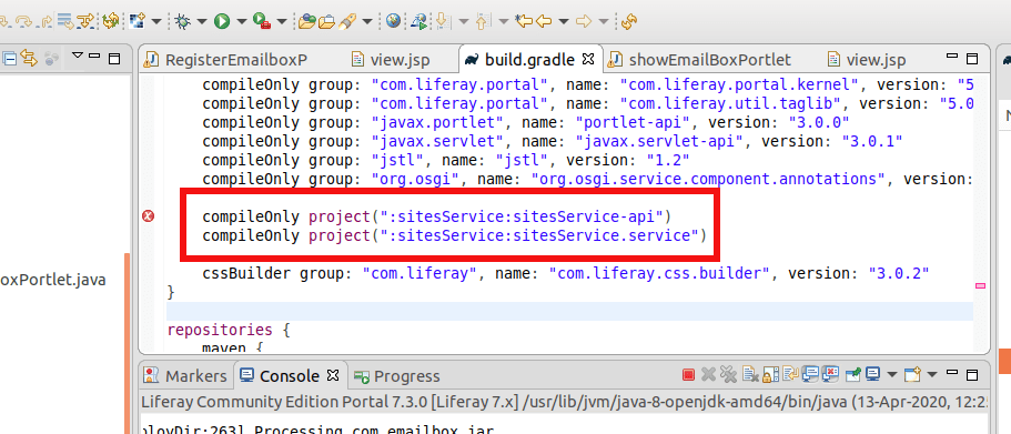
Could not run phased build action using Gradle distribution 'https://services.gradle.org/distributions/gradle-5.6.4-bin.zip'.
Build file '/home/abhilash/eclipse-workspace/register-emailbox/build.gradle' line: 32
A problem occurred evaluating root project 'register-emailbox'.
Project with path ':sitesService:sitesService-api' could not be found in root project 'register-emailbox'.
Several individuals have encountered this particular issue, and you can find detailed guidance on resolving it in the Liferay developer article focused on creating a service builder.
Through extensive research, I discovered that the solution to this issue requires creating both a portlet and a service builder within the Liferay workspace, rather than the Eclipse workspace. Specifically, it is essential to create a Liferay workspace project inside the Eclipse workspace to address this problem effectively.
Lets do that this time.
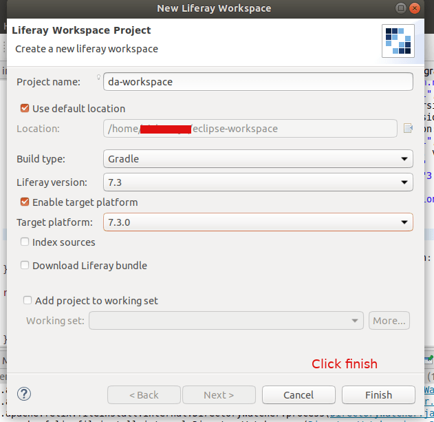
Click File -> New -> Liferay Workspace Project
Provide a Project Name and click on Finish
Next right click on the da-workspace, New -> Liferay Module Project
Provide the Project Name, then it automatically changes the Location Provide the class name and project name
Deploy this service by clicking on the gradle section of IDE and double click on deploy
Deployed successfully
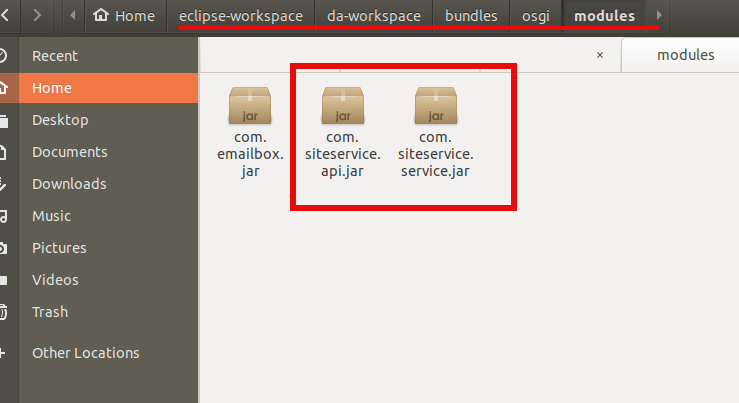
You can see the module os created inside our new Liferay Workspace: da-workspace
Jar file created
Copy this jar file and paste into the liferay server folder path given below:
2020-04-14 09:16:09.299 INFO [fileinstall-/home/abhilash/liferay-ce-portal-tomcat-7.3.0-ga1-20200127150653953/liferay-ce-portal-7.3.0-ga1/osgi/modules][BundleStartStopLogger:39] STARTED com.emailbox_1.0.0 [1117]
Status -> STARTED
Now delete our old services. Goto the Goshell and uninstal the bundles:
Now goto the liferay and check our newly created portlet
Now lets repeat the steps for creating the service-builder from the previous article. But this time create it from da-workspace
File -> New -> Liferay Module Project
Services are created – For details check the previous articleFolder structure for the portlet and the service builder
Add the details as shown in the below screenshots (If any doubt check the previous article).
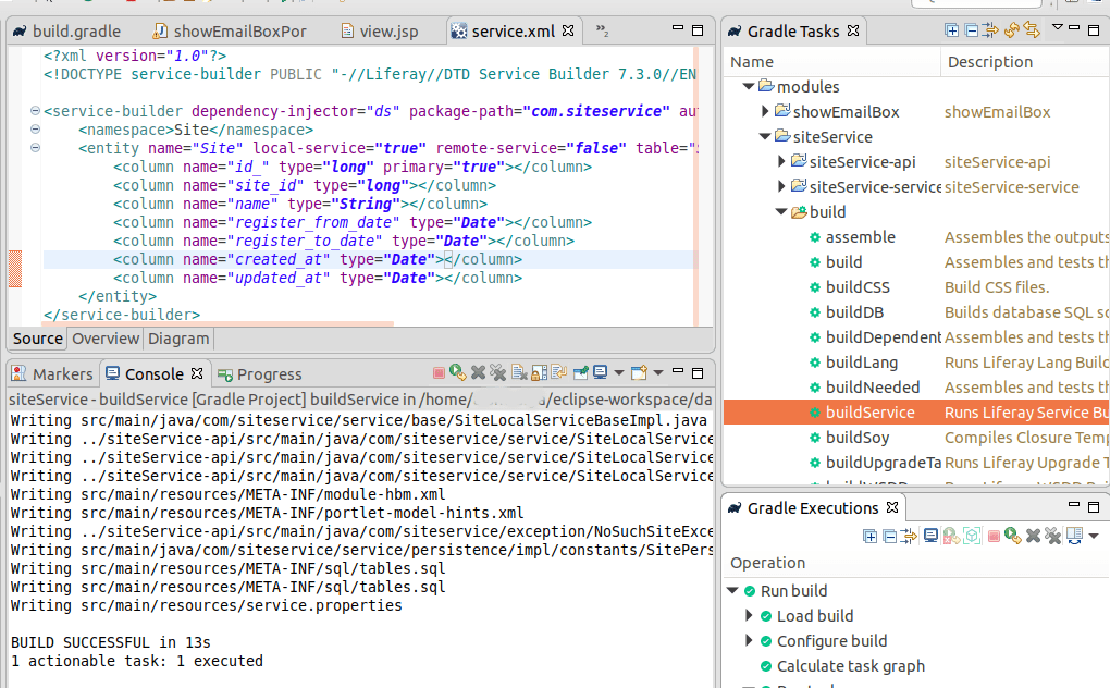
Do builder service and deploy
Copy this jar files one by one to the server’s deploy folder. First *api.jarand then *service.jar
Server logs:
liferay-ce-portal-tomcat-7.3.0-ga1-20200127150653953/liferay-ce-portal-7.3.0-ga1/osgi/modules][BundleStartStopLogger:39] STARTED com.siteservice.api_1.0.0 [1118]

liferay-ce-portal-7.3.0-ga1/osgi/modules][BundleStartStopLogger:39] STARTED com.siteservice.service_1.0.0 [1119]
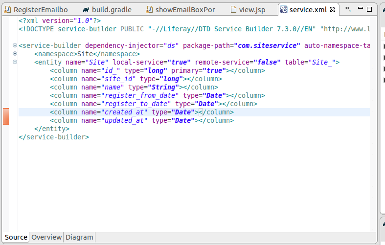
Check the database, you can see the Site_ Table and columns are created.
Now add the service builder dependancy to the portlet
Add this two lines in the build.gradle file
Right click on showEmailBox portlet and gradle -> refresh gradle project
DONE! You are successfully binded the service builder to your portlet.
now add the following to your portal class file above the doView function
But what is we needed to fetch suppose some sites which has particular site_id Or fetch all sites which has registered after this time etc?
For all these custom query to mysql db, we needed to create a custom finder methods. So lets create one.
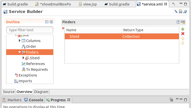
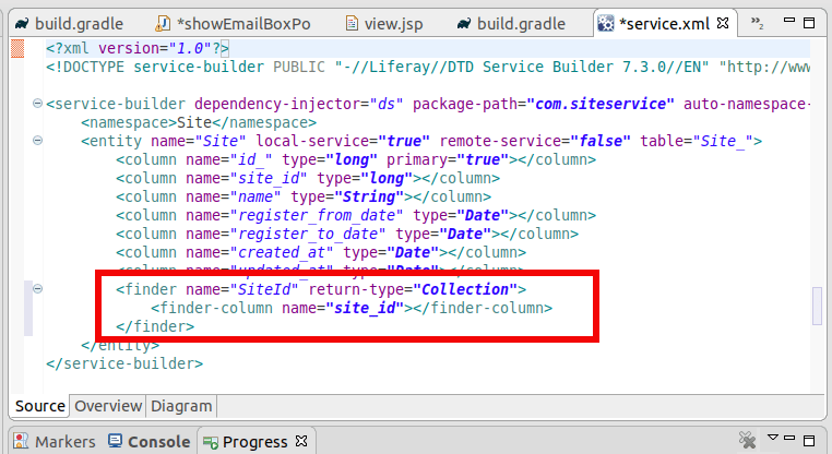
Open service.xml of `siteService-service`
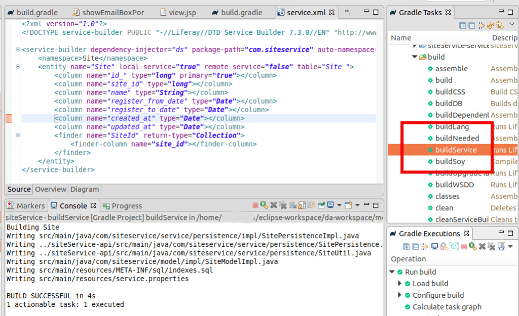
Click on Finders and add Name and TypeClick on Finder column and add the db column to findClick on Source, you can see the finder is addedDouble click on the buildService to build the service
Now we can add custom finder findBySiteId to this service.
Open siteLocalServiceImpl.java
package com.siteservice.service.impl;

import com.liferay.portal.aop.AopService;
import com.siteservice.model.Site;
import com.siteservice.service.base.SiteLocalServiceBaseImpl;

import java.util.List;

import org.osgi.service.component.annotations.Component;


@Component(
	property = "model.class.name=com.siteservice.model.Site",
	service = AopService.class
)
public class SiteLocalServiceImpl extends SiteLocalServiceBaseImpl {

	public List<Site> findBySiteId(long site_id) {
		return sitePersistence.findBySiteId(site_id);
	}
}
Now do the buildService for siteService. Then Gradle -> Refresh and deploy the service. Copy this jar files one by one to the server’s deploy folder. First *api.jar and then *service.jar
Refresh Gradle project for the portlet – showEmailBox
Add the following to the doView function of the portlet
Site site = _siteLocalService.findBySiteId(2233).get(0);

System.out.println("We got the site: ---------");
System.out.println(site);
and don’t forget to create a site entry in the database with id: 2233
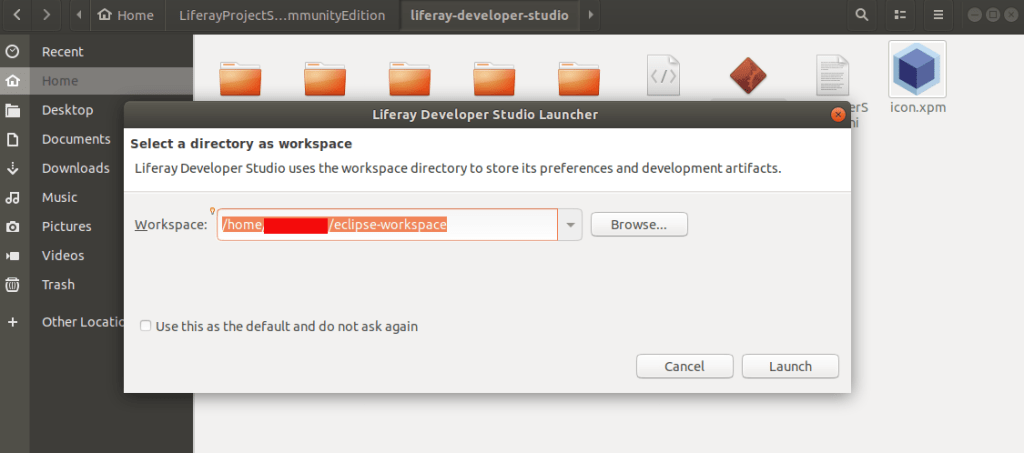
This is how Liferay Studio Workspace home page look like
You can create liferay plugins / projects etc from here.
Step 3. Click on right corner first button and open perspective.
select Liferay plugins
Open Perspective
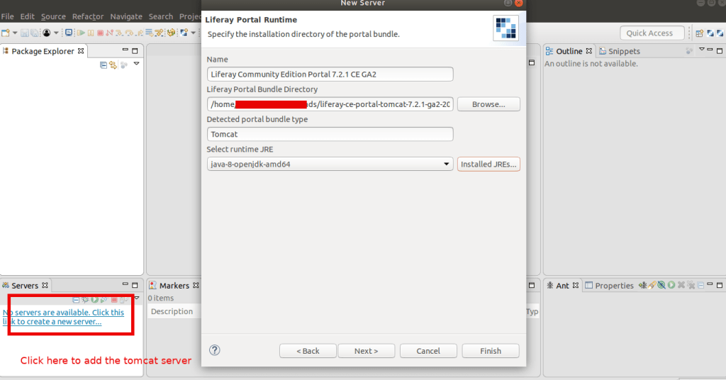
Step 4. Left bottom corner there is ‘Servers’ Tab
right click on it and select ‘New’ -> ‘Server’
Select ‘Liferay inc’ -> Liferay 7.x and click next
Add the tomcat server to your SDK to control the server from SDK. This helps you to see the server logs and other live status in IDE
Select the tomcat server path from your downloaded liferay portal
Make sure you are using the timestamp folder in the path of the server, else it not gonna work. It will show you an error like this:
If you start the tomcat server and try to access it without the timestamp PATH
You can add an existing resources created if available like theme etc to the server. If you don’t have any resources don’t worry. We are going to cover this in next chapter.
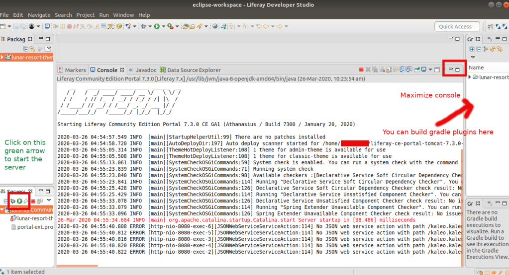
Click on the server name on the bottom left corner and you can see the configurations of the server.
Server Started. You can see the server logs in the console
I got this error after my thinking sphinx updation to the newest version of ‘3.0.5’. The error shows in the exact line of the code Model.search in my Rails controller. I updated my mysql2 version to ‘0.3.13’, and the issue is solved.
So in you Gemfile update the mysql2 version: